I was eight years old when my father graduated from college. He’d spent the better part of a decade working all day, going to school at night, and trying to manage three young boys somewhere in-between. I don’t remember when he found the time to do homework but I do remember that he had these really interesting magical-seeming books on his shelf or on his desk or on the kitchen table. Most of them were big and heavy with glossy pages and lots of pictures. Somewhere around the time I was nine or ten, my father handed me the smallest of these books, a thin, yellowed volume about the size and shape of a paperback and told me I should try reading this one. It was filled with many weird symbols and lots of black-and-white sketches of shapes and curves. It was called something like “Algebra and Trigonometry,” neither of which were words that I knew. He also gave me one of these:

And showed me how to use it to measure these things called “angles.” I remember leafing through this book and coming upon this really neat “fact,” namely that the sum of the measure of the angles in any triangle is 180 degrees. Now, this was interesting! I knew what a triangle was, I knew how to measure angles, and I knew how to add. This was something I could explore! So, dutifully, I began sketching triangles in my notebook, measuring the angles, and adding up the results. And, I quickly discovered something quite odd – my measurements didn’t always add up to 180. Sometimes I’d get 179.5 or 178 and sometimes 181 or 182. What, I wondered, was going on here? Was this magical book wrong? Had I discovered something new?

I remember showing my results to my father and him telling me it was my measurements that were wrong and imprecise. I wondered how he knew this and he explained that we don’t know that the sum is always 180 because we keep measuring triangles and discover this fact, but rather, we know this “fact” because of this thing called “proof.” It would be many, many years before I’d really start to understand this distinction but it’s this distinction I want to talk about here today and ultimately relate it to questions that seem to be swirling around concerning mathematical modeling and the notion of “real-world.”

Let’s continue to think about triangles. Here’s a triangle:

Now, the problem is that I’ve just lied to you. The thing that you’re looking at isn’t actually a triangle at all. Rather, the thing you’re looking at is a representation of the abstract mathematical concept of “triangle.” This is a fine distinction, but an important one. Triangles don’t actually “exist” in the same sense that my cat exists, or the sun exists, or a bottle of water exists. A triangle only exists as this abstract object that is brought to life by a mathematical definition. One example of such a definition is:

A triangle is a polygon that has precisely three sides.

Like all good definitions, this tells us the class of objects that our new object (triangle) belongs too, namely the class of things called “polygons,” and it tells us the specific difference between our new object and other elements of the class, “has precisely three sides.” The picture above is not a triangle, but rather is a picture of what one of these abstract things we call “triangle” might look like if we attempted to visualize it. But, and this is important, triangles themselves simply do not exist anywhere in this place we live, this place we call “the universe.” We can’t point to a triangle, we can’t draw one, we can’t pick one up, touch one, or taste one. They only exist in this abstract world that we call “mathematics.”

But, you ask, are triangles real? And, this is where the confusion begins. This is not an easy question. Plato believed that they were real and that somewhere there existed, in the same sense as my cat exists, this “abstract world of forms” populated by things like triangles and continuous functions and notions of “catness.” Plato believed that this abstract world of forms was the primary reality and that the world of substance and matter which we inhabit was but a mere shadow of this abstract world.

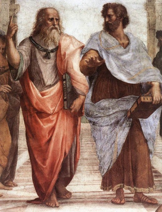
Of course, Aristotle disagreed and argued that no such world of forms existed and that our world of substance was the primary reality, that is, it was the world that my cat inhabits that is actually “real.” Plato and Aristotle’s disagreement sits in the center of the famous picture, “School of Athens” by Sanzio, which hangs today in the Vatican. Plato, on the left, points upward toward his “world of forms,” while Aristotle, on the right, points forward to what’s in front of us.

Now, what does all this have to do with mathematical modeling? Let’s go back to a definition of mathematical modeling put forth in the GAIMME report:

Mathematical modeling is a process that uses mathematics to represent, analyze, make predictions, or otherwise provide insight into real-world phenomena.

There is much debate and angst that arises around the very last part of that definition, namely the use of the term “real-world.” Some argue that triangles are “real” to children in a way that irrigation systems are not and hence conclude that doing any form of mathematics is doing mathematical modeling. This is, of course, where one falls into the trap of equivocation. In arguing in this way, one changes the meaning of “real-world” from indicating Aristotle’s world of substance and things to meaning “familiar to me whether it’s part of the world of substance or not.” This equivocation is the challenge and the fault. We need to use “real-world” in the sense that it’s intended by those who state definitions such as are found in the GAIMME report. We can’t arbitrarily change that meaning any more than we can change the meaning of “polygon” in our definition of triangle to include objects with curved sides and still expect our definition of “triangle” to make sense.

But, does this really matter? What’s lost if we change the meaning of “real-world” to be a subjective one that means “anything with which I’m familiar”? This is the truly important part. In making that shift, all is lost. All that is special, and powerful, and unique about this practice called “mathematical modeling” is dependent upon this connection to the “real world,” where here, the “real world” means the physical world, the natural world, Aristotle’s world of substance, or what we commonly refer to as the “universe.” The magic of mathematical modeling is that it connects Plato’s abstract world of forms (whether you believe in it or not) to Aristotle’s world of substance.

Mathematical modeling allows us to use the things we discover in the abstract world of mathematics to understand things in this other place, this space we inhabit, this non-abstract world of cats, and water bottles, and irrigation systems. The heart of mathematical modeling is the ability to bridge that gap, to make those connections, and to learn how to connect and use the abstract world to understand the world we inhabit. It’s the skills that are needed to work in that gap that is the new thing about teaching and learning mathematical modeling and that’s what we lose if we equivocate and redefine “real-world.”

The fact is that it is working in that gap that requires a new set of skills. And it’s this fact that makes the teaching and learning of mathematical modeling new and challenging. One must have an understanding of and be able to operate in the “mathematical world.” But, one must also have an understanding of and be able to operate in the “real world.” One must know or learn things about physics, or chemistry, or sociology, or farming, to be able to connect what they know in the mathematical world to this real world. One must learn how to make these connections, how to attach which abstract notions of mathematics to which phenomenon in this space we inhabit. One must learn the strengths and limitations of such connections and how to test them. Engaging in this practice or process and doing so in order to understand or make predictions about the “real world” is what we call “mathematical modeling.”


I couldn’t be in San Francisco last week for the Mathematical Sciences Research Institute’s workshop, “Critical Issues in Mathematics Education 2019,” which focused on mathematical modeling in the K-16 world. Fortunately, we no longer need to wait for proceedings to be published before we can share in such meetings and today, through Twitter, YouTube, and the MSRI website we can follow the discussion quite easily. On Thursday morning, there was an interesting panel discussion featuring Sol Garfunkel, Dan Meyer, Nina Miller, Annalee Salcedo, and Erin Turner that subsequently generated a lot of noise on Twitter and apparently a good deal of discussion at the meeting.

At the center of this noise lies the five minutes of remarks made by Dan Meyer which he has helpfully transcribed in full on his blog. At the start of his blog post Dan refers to the controversy and quotes a follow-up remark by Sol Garfunkel that’s worth repeating here:

So we might as well start this fight right now. I think Dan is completely wrong. The reason we wrote the GAIMME report was to put out a standard definition of modeling. Now you could use another definition. But the definition of mathematical modeling in the report and the one all the people I know who work in the field agree on is that it begins with a real-world problem.

Sol goes on to explain that definitions themselves are neither right nor wrong, they are simply useful or not. Of course, I agree with just about everything Sol said, except the “I think Dan is completely wrong” part. I think that doesn’t go far enough and that we’re better served by borrowing a description from the theoretical physicist Wolfgang Pauli who is said to have remarked upon particularly careless thinking by describing it as “not even wrong.”

Let’s take a look at Dan’s remarks and see if we can understand exactly where he went “not even wrong.” Dan starts out okay with the easy crowd-pleaser of criticizing a textbook problem labeled “CCSS Modeling” that well, clearly isn’t.

It’s worth noting that Dan doesn’t describe why he thinks this particular task isn’t mathematical modeling, but just takes his shot and moves on. One gets a first inkling of the “not even wrong” level of confusion here when one realizes that by Dan’s later definition of modeling, even this example is actually modeling. So, we started by criticizing textbook publishers for “calling any problem modeling for the sake of a good alignment score for their textbook” but later even this example is modeling? What? Okay, this is not going to be easy to untangle.

Dan’s next attack is aimed in a different direction, this time, at the authors of the GAIMME report. He claims that these authors have placed modeling on a mountain “that is far too high for any mortal teacher to climb.” His main critique here seems to be that the report is just too long. Two hundred whole pages! Who could read such a thing!? Forget for a moment the fact that this ignores entirely the “How to use this document” section of the GAIMME report which suggests that readers read the introductory chapter and then skip to the chapter on their grade band of interest, significantly shortening the reading time for any given individual. Instead, think about this claim – a 200 page document is simply too long for any practicing teacher to read in order to learn about a new topic with which they are unfamiliar and which they wish to bring into their classrooms. To me, this shows a stunning lack of respect for teachers as professionals. Dan, I think you could have looked to either your left or right and found teachers like Nina Miller and Annalee Salcedo sitting next to you who clearly would and did read the GAIMME report. I think we need to have more faith in teachers.

But, Dan’s just getting started and next he turns to an argument that looks as if it may actually have substance. He turns to the content of the GAIMME report and claims that it depends heavily on adjectives like “messy,” “open,” “real-world,” and “genuine,” claims that these adjectives have no shared meaning and concludes that the only way to know if something is mathematical modeling or not is to ask an author of the GAIMME report. One has to wonder if he’s actually read the report. On page ten of the GAIMME document we find this nice, succinct, relatively adjective-free definition of mathematical modeling:

Mathematical modeling is a process that uses mathematics to represent, analyze, make predictions or otherwise provide insight into real-world phenomena.

This is a nice definition. It tells us the class of things that mathematical modeling belongs too, namely those we think of as “process,” and tells us the specific difference between the process of mathematical modeling and all other processes. This process is one that uses mathematics in a particular way to uncover things about real-world phenomena. Large chunks of the rest of the document work to unpack and explore this definition and even to provide alternative, equivalent definitions, but I certainly don’t feel that I need to give Sol a call every time I want to check something against this definition.

But, this is still warm-up. Dan is just setting the stage for his new and improved definition of “mathematical modeling” which, wait for it, is “All learning is mathematical modeling.” So, I guess when my cat learns that the sound of a can opener means food is about to arrive implies that she’s doing mathematical modeling! Heck, this is easy! We don’t need to do anything at all to teach mathematical modeling, even a cat can do it! Let’s all just keep doing what we were doing, nothing more to talk about here.

This, of course, is really where Dan has his “not even wrong” moment. By ignoring (ridiculing?) the work that folks like Sol Garfunkel and others have done to attempt to define and explain this absolutely essential mathematical practice that yes, we call “mathematical modeling,” and by replacing it with “all learning is modeling,” Dan unfortunately engages in the worst possible form of equivocation. And, that’s a shame. Dan’s built a following because he’s said a lot of sensible and important things about mathematics teaching and learning. But, this time, he’s taken a wrong turn and gone down a road that I’m afraid leads to a dead-end. Not just for him, but for the students of teachers who follow him down that road. The fact is, mathematical modeling is an essential mathematical practice. It’s one that’s been practiced for hundreds of years. Galileo did it. Newton did it. Einstein did it. And, today, thousands upon thousands of scientists, engineers, mathematicians, economists, social scientists, finance professionals, data scientists, and countless others rely upon this practice to continually push forward our ability to understand the world around us. It’s not a simple practice. It’s harder than guessing the next number in a sequence and it’s different than making conjectures about polygons. But, it’s worthwhile, and I believe, it’s attainable for teachers throughout K-16 and their students. Today, there are more resources available than ever before to help teachers at all levels get started in the classroom. The GAIMME Report is a good start. Sol Garfunkel’s COMAP organization provides multiple such resources including the jointly sponsored Mathematical Modeling Hub. Heck, there are countless blogs like this one and folks across the country and across the K-16 spectrum working to develop new resources and working with teachers to support them in mastering and teaching the essential 21st Century skill of mathematical modeling. So, let’s put aside this “not even wrong” conception that “all learning is modeling” and focus on the real work and the real-world work that remains to be done.

John


Our posts this year have been a bit sparse as Michelle and I have spent most of our free time continuing work on Model with Mathematics, our text on the art of mathematical modeling under development with Math Solutions. But, I was inspired by the joint release of the position statement on STEM Education by NCSM and NCTM, and thought it was worth commenting on this very worthy attempt to bring some clarity and coherence to STEM education and especially to the role of mathematics in STEM education. The key position statement is brief and worth repeating here:

The National Council of Supervisors of Mathematics (NCSM) and the National Council of Teachers of Mathematics (NCTM) recognize the importance of addressing STEM fields (science, technology, engineering, and mathematics) in PK–12 education and affirm the essential role of a strong foundation in mathematics as the center of any STEM education program. In addition to integrative experiences connecting the disciplines of STEM, students need a strong mathematics foundation to succeed in STEM fields and to make sense of STEM-related topics in their daily lives. Thus, any STEM education program (including out-of-school activities) should support and enhance a school’s mathematics program, ensuring that instructional time for mathematics is not compromised. In addition, any STEM activity claiming to address mathematics should do so with integrity to the grade level’s mathematics content and mathematical practices.

While I’m not entirely sure that I would put mathematics at the “center of any STEM education program,” I absolutely applaud the notion that effective STEM education requires a strong foundation in mathematics and applaud the notion that any STEM education program should support and complement a school’s mathematics program. The argument put forth in this position statement is spot on – a strong foundation in mathematics is essential to STEM, either viewed from an integrative viewpoint or from a purely disciplinary viewpoint, and hence STEM education programs developed in schools should support the strengthening of this foundation.

The NCSM/NCTM document containing the position statement above expands upon this statement and contains a list of recommended action steps for policy makers, teachers, curriculum developers, and informal educators. Today, I want to look at a few parts of the remainder of the document in a bit more detail, expand upon a few points, and attempt to tie some of the thinking offered in this document back to the teaching and learning of mathematical modeling and some other ideas around STEM that we’ve previously explored in this space.

To me, a key part of the document is the section titled “Envisioning STEM Education.” This section asks and attempts to answer the key questions – What is STEM? and What should an effective STEM program look like? The authors outline and contrast the often conflicting viewpoints on these questions, ranging from the “anytime you’re doing any of the four disciplines you’re doing STEM” perspective of authors like Larson to the “STEM is an integrative meta-discipline” perspective that we’ve taken in this space in previous posts. I again applaud the authors of this document for finding an effective middle ground, essentially recognizing that the disciplines of S, T, E, and M provide the necessary foundation for integrative activities that comprise STEM and encouraging the development of STEM programs that do both. In the particular case of mathematics, that means encouraging STEM programs that both support the development of foundational mathematical knowledge and support integrative activities that involve multi-disciplinary and interdisciplinary thinking. My only criticism of this section is that I don’t believe that the authors push far enough regarding the nature of the role that mathematics should play in integrative STEM activities.

On this point, we find the authors stating:

Students may use mathematics or science to model problems from the aforementioned list as they develop creative approaches and solutions.

And:

When incorporating mathematics as part of a STEM activity, it is important to ensure that the mathematics is consistent with standards for the targeted grade level(s) in terms of content as well as the level and kind of thinking called for.

And:

An essential feature of integrative STEM activities should be that they support the individual disciplines addressed with integrity – using content from grade-appropriate standards that is taught in ways that support pedagogical recommendations from the disciplines.

I don’t disagree with any of these particular statements. They are all certainly important points, but I don’t believe they go far enough and I do believe they leave the door open to the continued development of what I see as particularly poor and in fact counter-productive STEM activities. The essential piece that I believe is still missing is the notion that in a truly excellent integrative STEM activity, knowledge and use of mathematics is essential for obtaining a solution. If students are simply asked to use mathematics to model some aspect of a STEM activity but do not need to use what they’ve learned through such modeling to achieve their goal, mathematics will continue to feel “tacked on,” and the centrality of mathematics to STEM will be lost. Yes, the level of mathematics should be consistent with grade levels and yes, the STEM activities should support the teaching and learning of the disciplines, but, integrative STEM activities should also allow students to experience and understand precisely why these disciplines are foundational and central to STEM. This is, of course, challenging and it requires the careful design of STEM activities that not only illustrate individually the central practices of S, T, E, and M, but also illustrate the connections and interplay between these practices that is indeed essential for addressing problems such as climate change, the spread of disease, or space exploration. Mathematical modeling, in particular, is not only something that can be done when tackling an interdisciplinary challenge like climate change, but something that often must be done to make sense of the world and to make progress on such challenges.

In the section titled “STEM in Schools” the authors of the position statement point out a particular and very real obstacle faced by the K-12 community in designing and implementing effective STEM programs, including STEM programs that provide activities that genuinely allow students to experience the importance of mathematics in STEM. They note:

In terms of instruction, many teachers coming from mathematics and science backgrounds may find themselves assigned as integrative STEM teachers, often without any relevant coursework or adequate professional learning to prepare them for such an assignment.

And:

Regardless, asking them to teach STEM in an integrative way without adequate background is likely to create new knowledge gaps and challenges and intensify the challenge of finding qualified teachers for mathematics and science classrooms.

Again, spot on. We know that most mathematics teacher education programs are not even designed to support teachers in the teaching and learning of mathematical modeling, let alone in the design and implementation of integrative STEM activities. We know that our mathematics teacher education programs are generally short on exposure to science and engineering. And, we know that there is sadly little to no time for practicing mathematics teachers to interact with and develop STEM programs and activities in conjunction with their science colleagues.

The NCSM/NCTM position statement ends with a set of “Recommended Actions.” I think these are excellent. I’d add a few more of my own though. Here they are:

Leaders and policymakers should:

  • Provide opportunities for professional learning, both for pre-service and in-service teachers, that supports mathematics teachers in their role in the development and implementation of STEM education programs.
  • Provide regular, structured, meaningful opportunities for mathematics and science teachers to learn together, work together, and experience the cross-disciplinary teamwork and collaboration expected of students in STEM activities.

Mathematics and teachers of STEM should:

  • Whenever mathematics is included in an integrative STEM activity, make sure that mathematics is essential for achieving the goal of the activity.
  • Seek and advocate for opportunities to collaborate with science colleagues to develop and implement cross-cutting activities in both science and mathematics classrooms that support STEM learning.

Program/curriculum developers should:

  • Develop truly integrative STEM activities and curricula that require and support the development of a strong foundational knowledge of mathematics and science and allow students to experience not only the practices of the disciplines but especially the interplay between those practices.

Again, I applaud NCSM and NCTM for their development of this position statement and for their efforts to bring clarity to STEM education and to the essential role of mathematics in STEM. This is a huge step forward, and I congratulate the authors on their excellent work. I look forward to future iterations and continued development of STEM educational activities and programs that supports the teaching and learning of mathematics and allows all students to experience the importance of mathematics and especially the practice of mathematical modeling in addressing the problems that surround us.

John


Some time ago, I had the pleasure of spending part of my summer working with a local high school teacher (Chuck Biehl), an undergraduate mathematics education major (Alexandrea Hammons), and a math education faculty member (Alfinio Flores), on a project we just called the “Bubble Board.” At the time, our interest was in developing a simple hands-on project that Chuck could take back to his classroom and where his students could gather data and learn a few things about curve fitting using a data-set they’d gathered themselves. We wrote this up as an article for the Ohio Journal of School Mathematics. You can find the full article here.

Today, I thought I’d revisit this project and talk a bit about it from the perspective of mathematical modeling. The Bubble Board is a great system in that it’s very simple to build and use, and in that students can gather data using nothing more than a stopwatch, a pencil, and paper. At the same time, the behavior of the system is interesting, and yet mathematically accessible for a wide-range of students.

The Bubble Board was originally designed by the physical chemist, Goran Ramme of Uppsala University in Sweden. Like many scientists before him, from Isaac Newton to Lord Rayleigh, Ramme’s been fascinated with soap films. It was from his wonderful 2006 book, Experiments with soap bubbles and soap films, that I first learned of the Bubble Board.

In designing the Bubble Board, Ramme was interested in devising a way to measure the average lifetime of a soap bubble. You blow a bubble and eventually it pops, but if you blow many bubbles and measure how long it takes each one to pop, what does the distribution of bubble lifetimes look like? Ramme’s Bubble Board gives you a way to blow a whole array of soap bubbles all at once. Here’s a picture of the version of the Bubble Board that we made:

As you can see, the system is simple. You have a latex sheet with an array of 56 identical, evenly spaced holes drilled into the sheet. Through each hole, you place a soda-straw so that about 2cm of the straw pokes through one side and the rest of the straw hangs below. The short end of the straws are then dipped, en masse, into a soap solution creating a flat soap film over the top of each straw. The board is then flipped and the long-end of the straws submerged in a water tank. The water, of course, rises in each straw and the resulting pressure “blows” a bubble at the other end of the straw. You end up with an array of identically-sized soap bubbles.

(Bonus Modeling Problem – How big will each soap bubble be? What is the relationship between how far you submerge the straws in water and the radius of each bubble?)

Now, Ramme approached the Bubble Board from the perspective above. That is, he approached the Bubble Board as a tool for measuring the lifetime of a large array of bubbles simultaneously, thereby building a picture of the distribution of bubble lifetimes and gaining insight into the average lifetime of a soap bubble. We approached the Bubble Board from the point of view of dynamical systems. That is, if you create this array of identical bubbles all at the same time, how does the population of bubbles evolve with time? Or, more simply – How many bubbles will be left at time t?

The dynamical systems perspective brings the Bubble Board into the world of population dynamics. This is of obvious interest in fields like ecology, where one wants to understand how the population of a given species, or group of species, changes with time. The study of population dynamics and the mathematical modeling of these types of problems has led to much beautiful and interesting mathematical work of broad applicability.

So, let’s think about the Bubble Board from this perspective a little bit and think about the Bubble Board from the point of view of mathematical modeling. When we first started building our Bubble Board and still hadn’t conducted any experiments, we reasoned as follows: “Well, if you have more bubbles at any given time, more are going to pop in the next instant of time, so the population of bubbles should decrease in a way that’s proportional to the population at any given time.” In other words, exponentially. That is, we argued that the rate of change of the total bubble population, P(t), should be proportional to the bubble population:

(1)   \begin{equation*} \frac{dP}{dt} = -r P(t) \end{equation*}

Here, r, is the rate of decay of our bubbles. Well, we’ve seen this equation before in this space and we know that the solution looks like this:

(2)   \begin{equation*} P(t) = P_0 e^{-rt} \end{equation*}

Here, P_0 
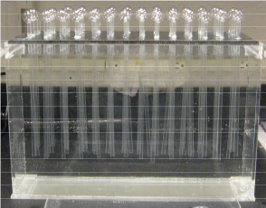
is the number of bubbles at time zero. So, we expected our bubble population to simply exhibit exponential decay. Then, Alex (Alexandria) went to lab and started measuring. Rather than the nice exponential decay we expected, Alex found this:

In this figure, the different colors indicate different types of soap solution, but here, let’s just focus on the purple or blue data points. Clearly, the data is not purely exponential. For some reason, the decay curve starts out somewhat flat and then exponential behavior seems to take over and drive the decay. Now, I haven’t put this discussion in the context of the modeling cycle, but hopefully you can see this as an example of how the cyclic nature of mathematical modeling arises naturally through comparison of model prediction and real-world data. We started with our hypothesis about how the system should behave, built our mathematical model and predicted a decay curve that was purely exponential. But, when comparing to the real-world, we see that we were clearly wrong! Well, we got the decay part right and part of the curve looks exponential, but certainly, there is some important behavior in our system that our model is not capturing.

So, we need to go back and revise our model and see if we can glean a deeper understanding of our system. Thinking about our array of bubbles a little more carefully we realize that if it’s true that bubbles have a common average lifetime, then near the start of the experiment very few bubbles should actually be popping. For example, if your average bubble lives for one minute, then near time zero, i.e. the start of the experiment, only a few “outlier” bubbles should pop. Most bubbles should persists and then as time gets close to one minute we should start to see your typical bubble pop. Here, the behavior should look like exponential decay as when your “average” bubble is popping, the number popping should be proportional to the number of bubbles you have. As you get well past one minute, you should again only see your “outlier” bubbles and they too should eventually pop.

How might we modify our mathematical model to capture this behavior? Well, in our original model we assumed a constant rate of decay. We called this constant r and said that for all time our population should decay at this fixed rate. But, now, we’re saying that for short times, this rate should be small and should increase to some constant rate only as time gets close to the average decay time of our bubbles. That is, our look at the data and our new hypothesis about how our population behaves implies a decay rate that varies with time rather than remains constant. Mathematically, we can achieve this by modifying our model like this:

(3)   \begin{equation*} \frac{dP}{dt} = -r P(t)(1-P(t)/M) \end{equation*}

If we think about this new term as being lumped together with the rate, r, that is, if we think about this as being our rate:

(4)   \begin{equation*} r(1-P(t)/M) \end{equation*}

then our rate of decay is small when the population is large, as we expect, and gets larger as the population shrinks. In fact, as the population shrinks, the new term becomes negligible and our model approximately becomes one of exponential decay. This new model is called a logistic model and the solution looks a little different than our previous solution:

(5)   \begin{equation*} P(t) = \frac{P_0 M}{P_0 + (M-P_0) e^{rt}} \end{equation*}

More importantly, the shape of the decay curve looks a lot more like the one we observed experimentally:

So, we can feel a bit more comfortable in that our model captures the real-world behavior more accurately. Of course, more work remains to be done! How, for example, does the constant M 
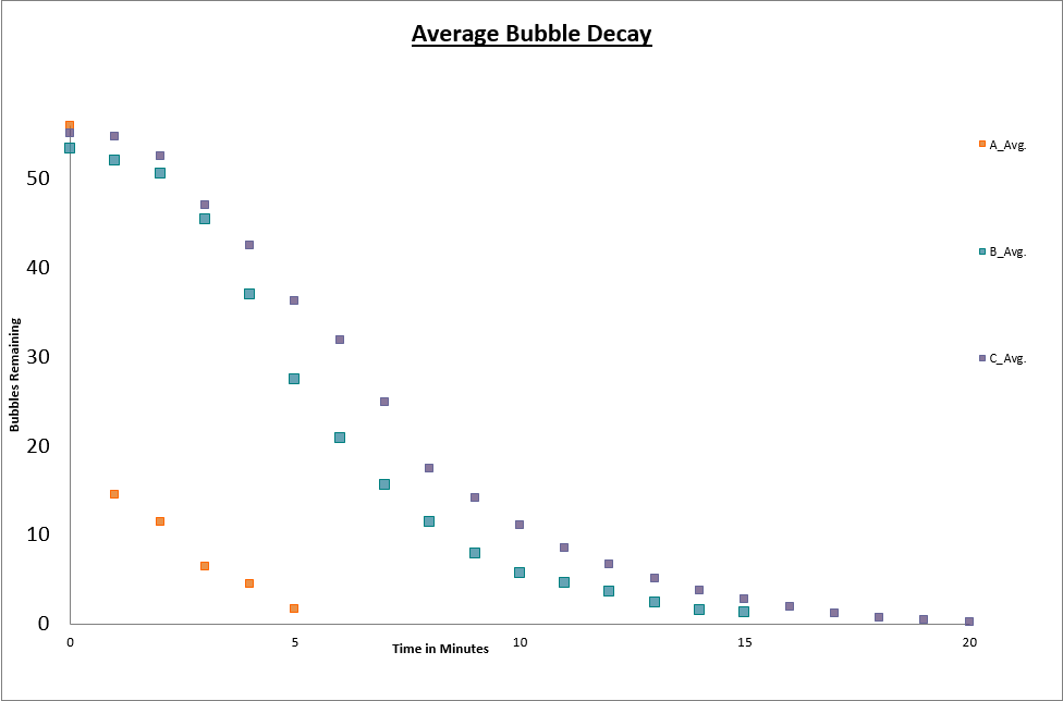
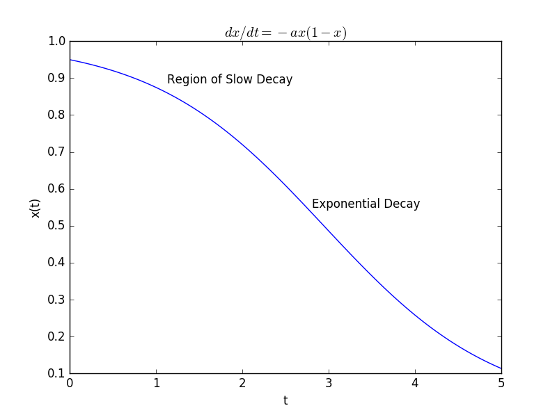
in our new model relate to properties of our soap bubbles? How does the constant r relate to these properties? Is there some reason to believe our variable rate is the right one?

Hopefully you enjoyed our detour into Ramme’s Bubble Board and can see it as a hands-on way to introduce your students to some interesting mathematical modeling questions and to the broader topic of population dynamics. The system lends itself to investigation by students across a wide-range of mathematical background, so whether you investigate the simple problem of predicting bubble size as a function of the depth the straws are submerged in the water, or the more complex problem of predicting how the population size changes with time, I think you’ll find something here to enjoy.

John


Well, the last few months of 2016 went by much too quickly and unfortunately left me with little time to post. But, it’s a New Year, and I’m anxious to get back to talking about mathematical modeling. So, Happy New Year! Now, let’s get back to work.

Recently, I found myself thinking about several points that we’ve explored in earlier posts. One of these, explored in “Caught or Taught?“, is the idea that mathematical modelers often draw upon a library of canonical mathematical models that they have at their fingertips when they approach a new problem. That is, they often reason by analogy, and use situations and models with which they are familiar as a starting point for thinking about new, unfamiliar, situations. The second point that’s been on my mind is the one explored in “Arduino as a simple tool for hands-on modeling activities,” and is the idea that the widespread availability of low-cost microcontrollers and sensors opens up new possibilities for hands-on activities in the modeling classroom. For many years at the University of Delaware, I’ve taught a mathematical modeling course where we’ve had students engage in hands-on experiments in our own laboratory. I’m constantly amazed that experiments which cost us thousands of dollars to perform just ten years ago can now be carried out at home on your desktop with just a few dollars in equipment.

So, today, I thought I’d explore a canonical mathematical model, but do it in a way that was hands-on and made use of accessible, low-cost technology. Along the way, I’ll point out some problems where you and your students can explore further. The basic mathematical model, exponential decay, is one with which you’re surely familiar, and is in-fact, one of the “starred” domains in the Common Core State Standards. Of particular relevance are the standards:

Distinguish between situations that can be modeled with linear functions and with exponential functions.

Recognize situations in which a quantity grows or decays by a constant percent rate per unit interval relative to another.

Interpret the parameters in a linear or exponential function in terms of a context.

To carry out this project, I enlisted the aid of my daughter, Julia, and this weekend, we spent time playing with potatoes. What more could a high-school student ask from their weekend? The question that we sought to answer was this – Which cools faster, a large potato or a small potato? Somewhat surprisingly, when we polled a few unwitting participants as to their answer to this question, two schools of thought emerged. One school of thought held that the small potato would cool faster as it “held less heat” and hence as it shed energy its temperature would drop faster. The other school of thought held that the large potato would cool faster as it had a larger surface area and that the rate of its losing energy would be hence be greater. Who’s right?

To explore this question, we decided we’d first build a mathematical model and try and make a prediction. Then, we’d design and carry out an experiment, compare, and see if we could both demonstrate an answer and understand why potatoes behave however they behave. For our model we were, of course, treading well-trodden ground. Examine the index of any introductory calculus textbook or any introductory physics textbook and you’ll find an entry for “Newton’s Law of Cooling.” Turn to the page referenced and in the calculus text, you’ll find yourself in the chapter or section on exponential and logarithmic functions. This goes back to our earlier point about canonical models. This mathematical model is certainly not new, but the idea that systems exhibit exponential growth or decay is so useful and encountered so frequently, that it is worth exploring models like these, deeply. So, without extensive derivation, here’s our mathematical model for the temperature of a potato:

(1)   \begin{eqnarray*} m c_p \frac{dT}{dt} = - hA (T-T_A) \\ T(0) = T_0 \end{eqnarray*}

Here, the unknown is the potato temperature, T(t). Room temperature is T_A and initially the potato is at some higher temperature, T_0. There are four parameters in the model. The mass of the potato, m, the specific heat, c_p, which measures the amount of energy needed to raise a unit mass of potato one degree in temperature, the surface area of the potato, A, and the heat transfer coefficient, h, which measures how fast the potato loses heat energy to the surrounding environment. We note that this model can be thought of as a statement of the principle of conservation of energy. The equation simply says the change in the energy of the potato is equal to the energy lost to the surrounding environment. The left-hand term is this change in energy, and the right-hand term relies upon Newton’s Law of Cooling which says that the energy lost to the surrounding environment is proportional to the difference between the temperature of the body and the temperature of the surrounding environment.

Now, we know that the exponential function is this very special function whose rate of change is everywhere proportional to itself. Our mathematical model says that the function we’re after, T(t), has this property that its rate of change is everywhere proportional to itself. Hence, our mathematical model is easily solved for T(t):

(2)   \begin{equation*} T(t) = T_A + (T_0 - T_A)e^{-\frac{hA}{mc_p}t} \end{equation*}

We see that the rate at which our potato cools is exponential, yes, but more importantly, how fast this decay happens for a particular potato is governed by the ratio of the four parameters in our problem:

(3)   \begin{equation*} \alpha = \frac{hA}{mc_p} \end{equation*}

Recall that we want to know whether a “big” potato will cool faster or slower than a “small” potato. The answer lies in interpreting our model and in particular, in interpreting \alpha
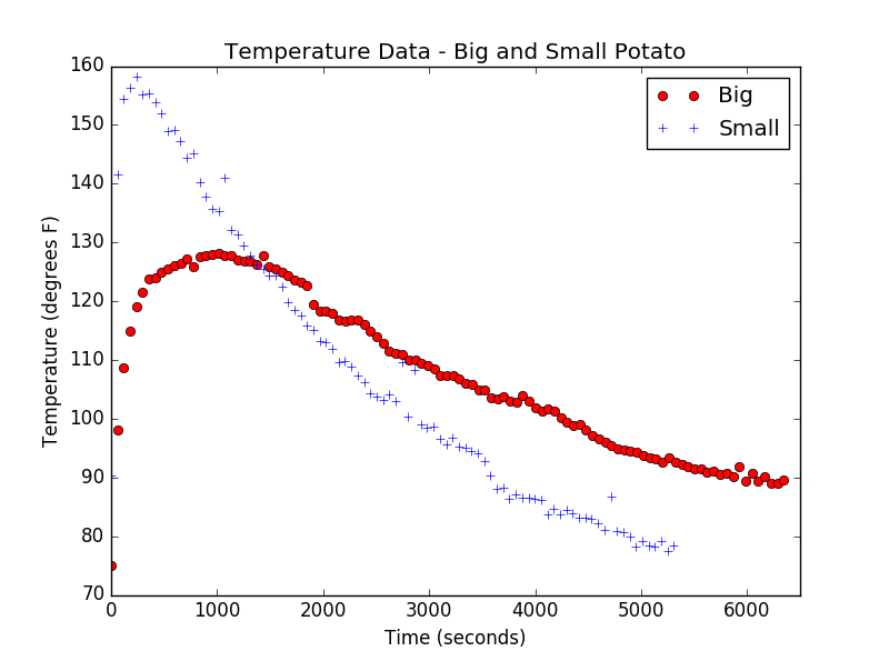
. For each potato, since they differ in mass and surface area, we’ll have a different \alpha. Suppose we call the \alpha for our small potato \alpha_S and for our large potato, \alpha_L.If we examine the ratio \frac{\alpha_S}{\alpha_L}, this ratio will give us our answer. If it’s bigger than one, the small potato must cool faster, if it is less than one, the large potato must cool faster. But, also notice that if we assume our potatoes are made of the same “potato-stuff” then h and c_p are the same for each potato, so this ratio only depends on a combination of potato masses and surface areas. In particular, this ratio reduces to:

(4)   \begin{equation*} \frac{\alpha_S}{\alpha_L} = \frac{A_S m_L}{A_L m_S} \end{equation*}

Here, the subscripts denote the small and large potatoes, as above. So, off to the supermarket we traveled where we bought two standard baking potatoes, one large, one small. The masses were easy to measure with our kitchen scale:

(5)   \begin{eqnarray*} m_S = 194.8g \\ m_L = 330.4g \end{eqnarray*}

But, how to measure potato surface area? (Here’s a problem for further exploration. How do you compute the surface area of a potato? How do you measure it?) I left Julia to tackle this question and she decided that this:

rather resembled this:

and after some measurements and computations arrived at:

(6)   \begin{eqnarray*} A_S = 137.13 cm^2 \\ A_L = 217.6 cm^2 \end{eqnarray*}

Putting this all together, we arrived at:

(7)   \begin{equation*} \frac{\alpha_S}{\alpha_L} \approx 1.06 \end{equation*}

and hence our mathematical model leads us to predict that this particular small potato should indeed cool faster than this particular large potato.

Our next step was to conduct some potato experiments. But, before we go there, let me point out another problem for future exploration. We’re making a prediction for our particular two potatoes. In this case, we predict that the small potato should cool faster than the large potato. But, is this always going to be the case? Surely, if we took our large potato and stretched it out into something resembling a giant French fry it would cool faster. Wouldn’t it? How does our ratio, \alpha, depend on potato shape? Can you find two potatoes that you would call “large” and “small,” where the large potato should cool faster?

Now, on to experimental potatoes. For our experiment, we used a low-cost microcontroller called a Particle Photon (\char36 19) and a TMP36 temperature sensor (\char36 1.50). We wrote Python code to carry out the sensing, gather data every minute, and store the data to a file for later analysis. This let us get lots of data for each potato, carry out the experiment over a long-time (one and a half hours), and not need to be there to monitor the experiment. If you’re interested, I’ve pasted the Python code at the bottom of this post for you to use or copy as you see fit. Now, if you don’t want to go the route of microcontrollers and sensors, all you need to carry this experiment out is a way to measure temperature and a watch. You could use a Vernier temperature probe or even a good old-fashioned glass thermometer. To heat our potatoes we placed each one in the microwave oven for five minutes. We then stuck our probe into the middle of the potato as best we could, sat back, and let our potatoes cool. Here’s our simple setup:
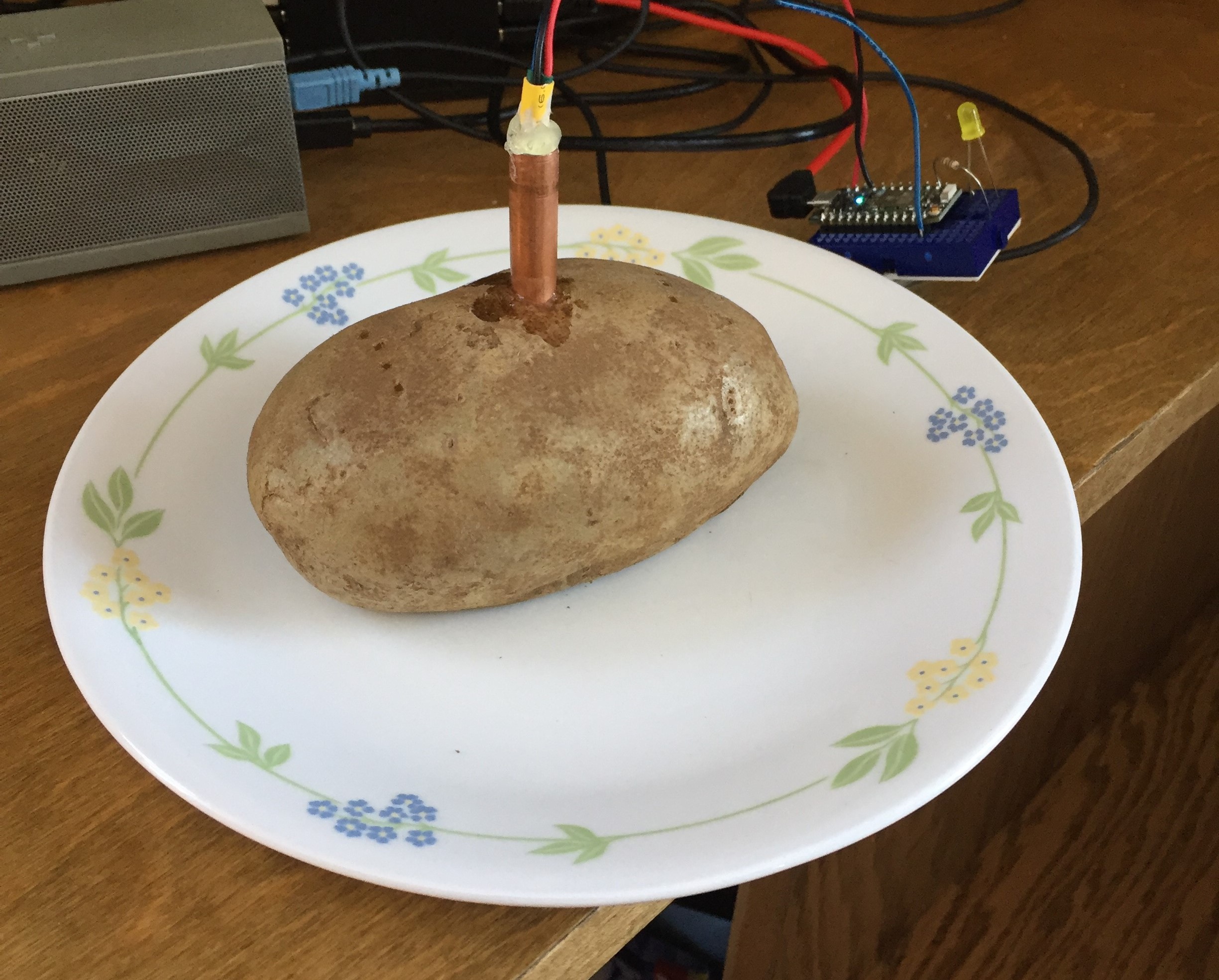
And, here’s our data:

As you can see, the small potato achieved a higher temperature initially, but, as predicted, cools at a faster rate. Since we placed each potato in the microwave for the same length of time and the small potato has smaller mass, it makes sense that its initial temperature should be higher. The transient behavior at the start also makes sense – it takes time for the probe to get to potato temperature. It’s exciting to see that our model and our analysis of \alpha yield a correct prediction about which should cool faster. By this point, Julia’s potato-patience was wearing thin, so we left further analysis for another day. But, here’s one final suggestion for exploration for you and your students. If you take the data above (or your own data) and fit an exponential to the exponential part of the curve, your fit will give you an experimental value of \alpha for that potato. If you take the ratio of the two values, how close do you get to 1.06?

Well, I hope you’ve enjoyed thinking about this canonical mathematical model and thinking a bit about hot potatoes. Best wishes for a fun year of mathematical modeling!

John


[code language="python"]
#Code for temperature monitoring using Particle Photon
#Using TMP36 temperature sensor with Photon
#Using standard wiring, red -> +3.3V, black -> GND, blue -> A0
#Reading is taken from A0 and converted to a temperature reading
#Note we had to install package spyrk via pip install spyrk

#Here is how to access the Particle Cloud

#Should be able to call via the access token for the system
ACCESS_TOKEN = 'YOURTOKENHERE'
#Or can use username and password
USERNAME = 'YOURUSERNAME'
PASSWORD = 'YOURPASSWORD'

#To create a connection to Python Code
from spyrk import SparkCloud
spark = SparkCloud(USERNAME,PASSWORD)

#Other packages we will need
import sys #Used to break the script if device not connected
import time #Used for delays and to assign time codes to data readings
import numpy as np #Used for creating vectors, etc. 
import statistics as stat #Used for computing median, etc.
import matplotlib.pyplot as plt #For plotting
import csv #For writing data to a csv file

#First we will test the connection to the device and terminate the script if not connected
#If connected we alert the user and continue
if spark.YOURDEVICENAME.connected != True:
 sys.exit("Device Not Connected")
elif spark.YOURDEVICENAME.connected == True:
 print("Device Connected")

#Now we will open a file for the temperature data
with open('temp_data.csv', 'w', newline='', encoding='utf8') as csvfile:
 filewriter = csv.writer(csvfile, delimiter=',', quotechar = '|', quoting=csv.QUOTE_MINIMAL)
 filewriter.writerow(['Time','Temperature'])
 
#Now we construct a function that will read A0 and return temperature
#Note the user calls this function by passing read_length which is the number
#of samples the function will take. The temperature computed from the median of these samples is returned to
#the user. That is, this function applies basic median filtering to the measurement. 
def read_temperature_F(read_length):
 work_space = np.zeros(read_length) #Creates an empty vector of length read_length
 for i in range(0,read_length): #This for loop reads read_length number of samples and puts them in work_space
   A0=spark.YOURDEVICENAME.analogread('A0')
   temperature = (9/5)*((A0*3.3)/4095 - 0.5)*100 + 32
   work_space[i] = temperature
 temperature = stat.median(work_space) #Finds median of readings and returns median value
 return temperature

 
#Now we want to set up a basic data gathering and plotting system for temperature readings
#We'll decide how many samples we want to take and how long between samples. Then, we'll gather
#those samples with time data as well and plot the temperature versus time
samples = 30 #We're going to take this many data points
time_delay = 55 #We'll allow time_delay seconds to elapse between measurements
temperature_data = np.zeros(samples) #Creates a vector for our temperature data
time_data = np.zeros(samples) #Creates a vector of same length for time

#This loop does the measurements
for i in range(0,samples):
 temperature_data[i] = read_temperature_F(8)
 time_data[i] = time.clock()
 print("Sampled temperature is", temperature_data[i], "at time", time_data[i])
 with open('temp_data.csv', 'a', newline='', encoding='utf8') as csvfile:
   filewriter = csv.writer(csvfile, delimiter=',', quotechar = '|', quoting=csv.QUOTE_MINIMAL)
   filewriter.writerow([time_data[i],temperature_data[i]])
 time.sleep(time_delay)

#Now, we plot the results
plt.plot(time_data,temperature_data,'ro')
plt.axis([0,time_data[samples-1],60,80])
plt.xlabel("Time (seconds)")
plt.ylabel("Temperature (degrees F)")
plt.title("Temperature Data - Particle Photon and TMP36 Probe")
plt.show()
[/code]

Today was the last day of this year’s NSTA STEM Forum and bright and early tomorrow morning I’ll be headed back to Delaware. I want to thank NSTA for a great conference and I want to especially thank all of those who joined me for one of our two NCTM workshops on mathematical modeling. I really enjoyed working with all of you and hope to have that chance again in the near future. I’ll repeat the offer I made at the end of each workshop this week – please feel free to tweet or email anytime with your questions, thoughts, or comments about mathematical modeling! I love thinking about this stuff and love hearing from math and science teachers working to implement mathematical modeling in their classrooms.

At this week’s STEM Forum there were a massive number of fascinating sessions offered. So much so that it felt like for each session I attended, there were a half dozen that I had to miss that I really wish I could have attended! So, today, for those of you who couldn’t join us for our NCTM workshops, I’ll give a brief recap and provide the slides and a few other related materials. Along the way, I want to share and explore some of the excellent thoughts and ideas offered by participants during and after these workshops. I apologize in advance for not having the foresight to write down names! If you recognize yourself below, please drop me a line and I’ll correct this oversight. One more stylistic note before we begin – our two workshops (middle and high school) were essentially the same, with the math explored in the high school session being slightly deeper than in the middle school session. So, below, I’ll just say things like “in our workshop” or “Our workshop began” for simplicity.

For easy reference, here’s a PDF of slides from our workshop: NSTA_STEM_2016_Pelesko_HighSchool

We began the workshop by sharing a short story that appears at the start of the physicist Eugene Wigner’s famous talk “The Unreasonable Effectiveness of Mathematics in the Natural Sciences.” I won’t reproduce the story here, but if you follow the link, we shared the first paragraph of Wigner’s talk. We then spoke briefly about this idea, the idea that there is this incredible power, a power that verges on the mysterious or miraculous, afforded to us once we understand how to use mathematics to understand the natural world. We talked about this as the basis for answering the question “How do we put the M in STEM?” and we asked participants to share their experiences and their challenges with incorporating mathematics into STEM activities.

Participants shared some very real and very pressing concerns that we need to overcome if we’re to be successful in putting the M in STEM and if we’re to be successful in implementing STEM overall. These included overcoming the discomfort that many math teachers feel with science and many science teachers feel with math. One participant noted that to overcome this, we need to find time and space for science and math teachers to collaborate and to work together. Absolutely! Another participant noted that if you looked at the NGSS and the CCSSM, they are almost forcing this to happen. These are excellent points and I want to emphasize them here – if we are going to effectively teach students the art of mathematical modeling, it is crucial that we learn to work across math and science. Yes, one can do mathematical modeling using contexts that require little understanding of science, but the full power of mathematical modeling is only really unleashed when we’re involved in a deep scientific investigation of phenomena in the natural world.

Next, we spent some time talking about the overlap in the practice standards between NGSS and CCSSM. In particular, we talked about SMP #4 – Model with mathematics, from CCSSM and Practice Standard #2 – Developing and using models, from NGSS. We spent some time exploring how the NGSS standard encompasses the CCSSM standard, with mathematical models being one type of model talked about in NGSS. The key idea we explored was this relationship, the idea that mathematical models are really scientific models encoded in the language of mathematics.

Then, we spent some time looking at a STEM activity and where mathematical modeling fit into the picture. The activity we discussed was the Great Lakes problem that I’ve talked about here. Participants spent some time working to construct a mathematical model of the Great Lakes system and at the end, shared their results and their thinking.

I want to mention two things shared by participants that I thought were really cool. One participant from Montana, told me about the Berkeley Pit Mine in Montana:

BP_02_0

Apparently, this is an abandoned copper mine, huge in scale, that is slowly filling with water. The problem is that the water is incredibly contaminated and that eventually the water level will rise to the level of the local water table. When that happens, backflow will occur, contaminating local and regional water supplies. This is clearly a source of many wonderful STEM and mathematical problems. I’ll think about this one some more and I’m sure will post more about this one. Thanks for sharing!

Another problem shared by a participant, was one she does in her class. In this project, she has students read the book “The Immortal Life of Henrietta Lacks” and then explore changing concentrations of drugs in the body. As her experimental system, she has students start with a beaker filled with water and a certain amount of dissolved salt. They measure the mass of the system, then remove a small quantity of the “drug filled water” and replace it with an equal amount of clean water. Then, they measure the mass again and repeat. Tracking the mass measured each time, they uncover the curve that describes the changing concentration of the “drug” in the system. Mathematically, this is identical to the Great Lakes problem we explored in this session and a great example of the generalizability of mathematics. That is, we often discover that mathematical models we’ve built of one system are able to describe what we see happening in lots of systems. This happens when the underlying processes are the same, as they are here. Again, thanks for sharing!

Thanks again to everyone who participated this week! Please feel free to email or tweet anytime! Looking forward to more great conversations about the art of mathematical modeling.

John


This week, I’m in Denver Colorado for the 5th annual STEM Forum and Exposition organized by NSTA. Later this week, on behalf of NCTM, I’ll be running two short “NCTM sessions” on mathematical modeling. In these sessions, we’ll explore the question “What should the “M” in STEM look like in a good STEM activity?” Later this week, I’ll post more about these sessions and the STEM forum, but today, I want to talk about my plane ride.

No matter how often I fly, I find that looking out the window of an airplane never gets old. Given a choice, I always choose a window seat, even if it means seat 35F at the very back of the plane as it did yesterday. My choice was rewarded with a cloudless sky for most of the flight and I spent my time alternating between reading and looking out of the window. Now, if you fly from Philadelphia to Denver, or fly any other route that takes you across the mid-west you’ll see large swaths of the country that look like this:

wuir-centerpivot-aerial-large

Crop circles! Well, okay, that’s probably not the kind of crop circles you thought of when you read the title to this post. But, they’re still really cool and it’s fascinating to see the patterns laid down over thousand and thousands of acres of the United States. These crop circles are, of course, the result of what’s called “center pivot irrigation.” This is where a pumping system is built at the center of a circle, a long mobile arm of sprinklers is constructed, and this arm pivots around the central pump, irrigating a large circle of crops. If you’ve ever driven through regions where center pivot irrigation is used, you’ve likely seen the sprinkler arms:

center-pivot-sprinkler-image-300x172

Flying over thousands and thousands of these crop circles yesterday, I realized that there are all sorts of interesting mathematical modeling and generally more STEM questions that they present. Here are just a few that occurred to me:

The pivot arm is on wheels all along its length. At various points along this radius, motors of some sort drive the motion. Since this is a radial motion, the motors furthest out must be going faster than the motors closest to the pivot point. How is this motion coordinated? How does this need to increase the motor speed with radial distance impact the largest such circle that’s practical?

Since water is being forced from a central point, the water pressure must drop as we move outward along the radial arm. This means that if all sprinklers were identical along the arm, the crops closest to the pump would get over-watered, and those furthest out under-watered. How does one design a sprinkler system for this arm so that we deliver the same amount of water across the entire circle?

While the arrangement of these crop circles clearly must follow, to a certain degree, local topography, why are they generally arranged in a less-than-optimal packing arrangement? That is, we know that hexagonal packing of circles covers more area than the rectangular packing we observe. So, why do these circles generally follow the arrangement on the left rather than the right in the picture below?

CirclePacking_1000

Why are the circles that we see generally all the same size? For the most part there are only two sizes of circles one will see. Why does there appear to be a minimum circle size? We know that if we used circles of various sizes, we could cover more area as in this picture:

circle-packing-574x347

Why don’t farmers use circles across a greater range of sizes?

Now, as with any good mathematical modeling problem or any good STEM problem, I imagine that the answers to these questions are complex, and involve multiple factors and multiple constraints. As my flight neared Denver yesterday though, I decided to see if I could at least convince myself that there was a good reason why we don’t see small crop circles by sketching out a really simple mathematical model. This was a “back of the airplane menu” type model, but nonetheless, fun to play with and I thought I’d share it with you here today.

I wanted to see if there was an economic reason why we don’t see circles below a minimum size. That is, are circles below a certain size just not profitable? I assumed that there were three basic costs associated with constructing and running a single center pivot irrigation system:

    \begin{equation*} C_p = \text{Fixed cost of purchasing a pump} \end{equation*}

    \begin{equation*} C_m = \text{Cost of water used, proportional to square of the radius of the circle} \end{equation*}

    \begin{equation*} C_r = \text{Cost of pivot arm, proportional to radius of the circle} \end{equation*}

I also assumed that the revenue one would generate was proportional to the area of the circle:

    \begin{equation*} R = \text{Revenue, proportional to radius squared} \end{equation*}

Putting this all together meant that the profit, P, could be written as:

    \begin{equation*} P = R-C_p-C_m-C_r \end{equation*}

Using my assumptions of proportionality to the radius, r, I could rewrite this as:

    \begin{equation*} P = a_0 r^2 - C_p - a_1 r^2 - a_2 r \end{equation*}

Here, the a_i are positive constants of proportionality. A little rearrangement yields:

    \begin{equation*} P = (a_0-a_1) r^2 - a_2 r - C_p \end{equation*}

Now, a_0-a_1 must be positive, otherwise, the profit would always be negative and there would be no sense in ever having any sort of circle. Knowing that means the general shape of the profit curve as a function of r must look like:

IMG_0372

The fact that this curve becomes positive only at some finite positive value of r means that, yes, there is a minimum size below which a crop circle just isn’t profitable. I’m convinced that our farm industry knows what it’s doing when it avoids making teeny-tiny circles. In fact, it seems that we should be driven to make our circles as large as possible (note that real circles cover hundreds of acres) and that there must be another explanation for why we only make them up to a certain size. I suspect that the maximum size of theses circles is dictated either by the demands of designing for the pressure drop across the sprinkler array or the demands of increasing speed of the motors as we move further out along the arm. Or, probably both.

But, it was time to ask my neighbors to get up one last time so I could use the bathroom and then, quickly, my plane ride to Denver was over. I hope you’ve enjoyed my random flight musings and hope perhaps you’ve found some inspiration for some cool STEM problems here in this post. I’ll be sure to post again at least once more this week and share what I learn at this year’s STEM Forum. Till later.

John


This post was inspired by a recent twitter conversation between @woutgeo, @ddmeyer, @cheesemonkeysf (cool handle!), and myself. The 120-character at a time conversation revolved around a comment from @woutgeo:

“…am still mulling whether modeling Q’s can have correct, known answers”

Since this seems to be a common point of confusion, or even contention, I thought I’d talk about this idea a little today. That is, what do people mean when they make statements like “Modeling problems don’t have a single, unique, correct answer.”? If you read the introductory chapter to the new Annual Perspectives in Mathematics Education (APME) volume, Mathematical Modeling and Modeling Mathematics, you’ll find versions of this statement in several places. I’ll highlight two:

There are multiple paths open to the mathematical modeler, and no one, clear, unique approach or answer.

Mathematical modeling authentically connects to the real world, starting with ill-defined, often messy real-world problems, with no unique correct answer.

What do people, in particular, what do those of us who do mathematical modeling professionally, mean by such statements? What are we really trying to say with statements like “no unique correct answer”? There are actually multiple levels to this point, and I think it is worthwhile exploring a few of these levels here today.

At the simplest level, such statements express the point that the answer to a modeling problem is not like the answer to a typical textbook or classroom math problem. When we think of the idea of an “answer” to a math problem, due to many years of repetitive training, what we most often visualize is a number. “The” answer is 586, or 7, or 2+3i, or \sqrt{17}, or something like that. Perhaps, if we’re a bit more deeply immersed in algebra, or trigonometry, or calculus, our default vision of “answer” might be more like x^3 or \sin(3 \theta) or \frac{1}{x} or some such expression. Note that this default vision of an “answer” is some form of mathematical object and tied to that, perhaps so intimately that we don’t see it, is the idea that this answer is easily checked. It’s the result of “doing the math correctly,” and hence, of course, we should only get one such answer. But, when we talk about the answer to a modeling problem, these are not the types of objects we’re talking about. In one very important sense, the answer to a modeling problem is a model. And, here is the first place where this idea of “no unique answer” comes into play. Because models of a given real-world situation can be constructed using wildly different mathematical tools and are based on assumptions made by the modeler, it is often the case, likely even, that two modelers approaching the same problem produce different models, i.e., different “answers” to the same modeling problem. This is the point that the first of the two statements from the APME volume above is really making.

But, there is another level to this idea of “no unique answer” that’s worth exploring. The second statement from the APME volume mentioned above points to this next level. Let’s examine the statement again:

Mathematical modeling authentically connects to the real world, starting with ill-defined, often messy real-world problems, with no unique correct answer.

Here, note that “answer” is not referring to the answer to some modeling problem in the sense discussed above, but is referring to the “answer” to a real-world problem that the modeler is trying to address. Here, the notion of “no unique answer” points to the messiness and inherent uncertainty of the real-world. Because we can never hope to capture all of that messiness or tame all of that uncertainty, our models always remain provisional, approximate, and open to improvement. That is, we obtain “an answer” to our problem, and we evaluate whether or not it is good enough for our purposes, but we never get “the answer.”

Another way to see this is to always keep in mind that mathematical modeling is ultimately, a process. Hopefully, it’s a process that draws us closer and closer to the truth, but like an asymptote, never quite gets there. You can see this point of view and get a sense of the notion that there isn’t one right “answer” or model, but rather a never-ending array of possible “answers” or models, in the CCSS for mathematics:

In situations like these, the models devised depend on a number of factors: How precise an answer do we want or need? What aspects of the situation do we most need to understand, control, or optimize? What resources of time and tools do we have? The range of models that we can create and analyze is also constrained by the limitations of our mathematical, statistical, and technical skills, and our ability to recognize significant variables and relationships among them. 

There is a wonderful one-paragraph story by Jorge Luis Borges that is related to this second point. It’s called “On Exactitude in Science” and in this story, Borges explores the idea of modeling and uses absurdity to remind us that useful models are always incomplete. His story is short enough to reproduce here:

In that Empire, the Art of Cartography attained such Perfection that the map of a single Province occupied the entirety of a City, and the map of the Empire, the entirety of a Province. In time, those Unconscionable Maps no longer satisfied, and the Cartographers Guilds struck a Map of the Empire whose size was that of the Empire, and which coincided point for point with it. The following Generations, who were not so fond of the Study of Cartography as their Forebears had been, saw that that vast map was Useless, and not without some Pitilessness was it, that they delivered it up to the Inclemencies of Sun and Winters. In the Deserts of the West, still today, there are Tattered Ruins of that Map, inhabited by Animals and Beggars; in all the Land there is no other Relic of the Disciplines of Geography.

The point, of course, that Borges is making is that a big part of science, a big part of understanding the real-world, is about making models and that the only perfectly complete model of reality is reality itself, but that such a model is also completely useless! This is true whether we’re talking about physical models like maps or more abstract mathematical models. The magic is that maps and models, approximate, imperfect, and ignoring vast parts of reality are incredibly useful and are our best tools for understanding, predicting, and controlling that reality.

John


Just spent a great week at NCSM 2016 in Oakland, CA. Wish we could have stuck around for NCTM 2016 across the bay, but sadly, not in the cards this year. Today, I thought I’d share a bit about our session on mathematical modeling for those who couldn’t be there in person.
First, let me share links to a few things. A PDF of our slides from the session can be found here.
We also left the attendees with two handouts that can be found here.
The first handout outlines the key features of mathematical modeling and the key features of the QFT, which I’ll talk about below. The second is a useful worksheet for helping teachers and students engage in meta-thinking about their mathematical modeling work.
During the opening of our session, Michelle strove to make the following point – it’s not surprising that teachers in the United States are finding the implementation of SMP #4 to be a challenge. She shared the following table which highlights the very small fraction of teacher preparation programs that provide their students with any training in mathematical modeling.
 Picture2(Newton, Maeda, Alexander, Senk, 2014, Notices of the AMS)
For teachers graduating from one of the 85% of programs that provide no training in mathematical modeling, preparing to teach SMP #4 is like preparing to teach geometry, never having had a course in geometry. In fact, it’s a bit more difficult, since even if someone somehow missed out on a college level course in geometry, they still would have seen it in high school. With modeling, we face the situation where the vast majority of teachers have never seen mathematical modeling at any level in their education. In addition to this issue, Michelle also discussed the huge deficits in secondary mathematics curricula related to mathematical modeling and made the point that a long history of embedding math tasks in pseudo-contexts has left students unprepared to deal with real real-world situations in the math classroom.
In the next part of our session, I spent some time discussing the points we discussed in one of our previous posts. Since at least one of the attendees found a new analogy we used particularly compelling, let me elaborate on that point here (thank @mary_davis_utdc!). When talking about the important fact that mathematical modeling is an iterative process, we discussed the question as to what exactly drives that iteration. For an analogy, I relied on one my favorite things, the lazy river. A special thanks to @mary_davis_utdc for tweeting us this picture after the session!
Cf8YwoZUYAAyq9e
In a lazy river, you’re just drifting around and around a river in a closed loop, that is in a cycle. But in every such river, at some point along the cycle, you’ll find there are jets that propel the water in a particular direction and keep the cycle moving. In mathematical modeling it’s the “Validate” step that serves as the “jets” of the modeling cycle. Remember, the “Validate” step is where you take the model that you’ve formulated and analyzed and compare its predictions or insight back to the real world. To the extent that your model’s predictions or explanation differs from what you see in the real world, you’re propelled (jetted?) back around the modeling cycle, back to the formulate stage, back around the lazy river of mathematical modeling. If this isn’t occurring, if you’re modeling activities aren’t being driven naturally around and around by this validation step, you’re not really doing mathematical modeling.
In the final part of our session, Michelle introduced a pedagogical tool that we’ve found particularly useful when engaging teachers and students in mathematical modeling. This is a tool called the “Question Formulation Technique” or “QFT” for short. It was developed by Rothstein and Santana over the course of many years and has been used in an incredibly wide variety of settings. I encourage you to visit www.rightquestion.org to learn more, or better yet, read their really excellent book on the topic:
 Picture3
Over the past several years, we’ve worked to find effective ways to incorporate the QFT into the teaching of mathematical modeling. The genesis of this idea was my stubborn insistence on defining mathematical modeling as “the art of asking good questions” and Michelle’s equally stubborn insistence on saying “What the hell does that mean?” As we thought about this carefully, we gradually realized that students often struggle with mathematical modeling in the same way that they struggle with mathematical proof – they’re stuck at the beginning, stuck at “Where do I start?” With modeling, clearly defining the questions your’re trying to answer, learning to identify the types of questions that modeling can answer, and identifying the questions you need to answer in order to build a model are all crucial steps. These occur right smack at the start of the process, somewhere within that “Problem” box and along the way to that “Formulate” step. What we’ve found is that using the QFT at the start of the task, or strategically at points along the modeling cycle, is a really good way to get students to think deeply about these questions, own these questions, and be motivated to answer these questions.
If you’d like to read a little bit more about our work with the QFT and mathematical modeling, here’s a draft article we’ve been working on.
My guess is that this isn’t going to make it much past the draft stage, as we’re now shifting to work on our new book on mathematical modeling. Ah, that’s a perfect segue to what was the biggest highlight of the week for us – signing a contract with Math Solutions to publish this book. It’s tentatively titled “Model with Mathematics” and we’ll keep you posted on progress here. We’re both very excited to be working with the Math Solutions team on this project and looking forward to sharing more of what we’ve learned about learning and teaching mathematical modeling with the community. So, stay tuned!
Finally, just wanted to say a special thanks to everyone who attended our session. What a great crowd! As always, please feel free to contact us with any follow-up questions or comments. We’d love to hear from you.
John

If there were a top-ten list of “things that make math teachers cringe,” the question “When will we ever use this?” would surely be at the top. That’s pretty independent of whether you teach at the elementary grades, middle school, high school, or college. Quite rationally I suppose, most students want to know there is some utility in what they’re learning, that this lesson is not just another “eat your spinach, it’s good for you” type of lesson, but is something they’ll be able to see as relevant to their own lives and their own careers.

One of the nice things about teaching mathematical modeling is that it’s incredibly relevant in a wide variety of contexts and to people working in a tremendous variety of fields. As I read the news each day, I keep an eye out for neat places where mathematical modeling shows up and today, I thought I’d share a few recent ones with you.

One of the coolest is the recent discovery of evidence for the existence of a ninth planet (poor Pluto!) in our solar system. This discovery, announced by Caltech researchers in January of this year relies entirely on indirect evidence provided by a mathematical model. In this case, no one has actually seen the ninth planet, all of the evidence comes from observations of objects in what is known as the Kupier Belt. These objects are moving in ways that just don’t make sense…unless there is some other very large mass out there as well. By constructing a mathematical model of how these objects should move and inserting an unknown large mass into the model, the Caltech team has shown that the most likely explanation for the motions that are observed is the presence of something that isn’t observed, i.e. a ninth planet. How cool is that? Note that the reasoning of the Caltech team is exactly the same as the reasoning we’ve been discussing here. They observed a pattern, they sought to explain that pattern, they made a hypothesis about what could be causing that pattern, they built a mathematical model incorporating that hypothesis and showed that the model predicted the observed pattern, and hence can claim that the probability that their hypothesis is true is now very high. In this case their hypothesis happens to be the very exciting one that a previously undiscovered planet exists!

In an entirely different direction, a team from the University of Aberdeen recently built a mathematical model that explains how things go viral. In this case, the team wanted to understand how things like the Macarena could suddenly become wildly popular, or how “Numa Numa” could garner more than two million views on YouTube in just three months, or more importantly how social movements, ideas, or products could catch on or fail to do so. Here, the team borrowed from mathematical models used in epidemiology, similar to those we explored in “Pictures and Stories,” and  added in the effects of acquaintances, such as those we maintain through social media, to construct a new model that could examine the spread of ideas. The Aberdeen team showed that while an individual’s resistance to the spread of a “contagion” might be high, when bombarded by that contagion from many directions, such as happens through FaceBook or Twitter, transmission occurs, i.e. you go view Numa Numa as well. That synergy leads to explosive transmission and we say that something has gone “viral.” This is not only a wonderful example of the use of mathematical modeling to explain a real-world phenomenon, but also a wonderful example of the generalizability of mathematics and mathematical models. The same mathematics and the same types of mathematical models that can be used to study the spread of Ebola here have been used to study the spread of ideas.

Another example that caught my eye recently was work that appeared in PLOS One, where researchers investigated the impact of deploying a test for a type of drug-resistant tuberculosis. The question here was whether or not having a test that detected the particular drug-resistant strain, in addition to existing tests for TB and another type of drug-resistant strain, would impact the spread of TB throughout a population. Knowing the answer to this question allows researchers to effectively direct their time and resources. If this third test would help contain the spread of TB, it would be worthwhile, but if it didn’t, that time and money could be more usefully directed toward something that would actually save lives. The answer here, arrived at through extensive mathematical modeling, was surprising. The additional test did nothing to impact the spread and hence is not worth developing or deploying. As you might imagine, this is the type of question that not only can be answered by a mathematical model, but can only be answered by a mathematical model.

Discovering new planets, explaining the spread of viral videos, and determining where to invest time and money in medicine, are just three very recent examples of mathematical models and mathematical modeling impacting lives and people around the world. I encourage you to keep an eye on the news; I’m certain you’ll quickly collect your own stable of such stories to share with your students when they ask you “When will we ever use this?”

John