If you spend any time reading the literature on mathematical modeling, you’ll quickly encounter some version of the phrase:

We build mathematical models of the real world in order to explain, predict, or control. 

Usually, you’ll find such language as part of a definition of mathematical modeling or of a fairly high-level description of the process. But often, this language isn’t revisited when examples of mathematical modeling are described. This language is often left by the wayside and it’s up to the reader to puzzle out what a given mathematical model was intended to do. Once you have some experience, this isn’t hard, but for the novice, it can be confusing and since the whole point of mathematical modeling is to accomplish one or more of these three goals, it is important for the new modeler to develop some facility with these concepts. So, today, I thought we’d explore the ideas of “explain, predict, or control,” and give concrete examples of each case. Hopefully this will help clarify these purposes of mathematical modeling in your mind and give you a framework for thinking about the purposes of your modeling activities in new cases.

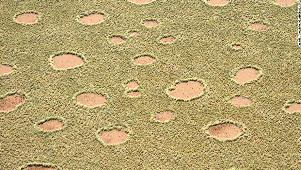
Let’s start with the notion of constructing a mathematical model to explain. This is the case that is most clearly and directly bound together with the scientific process. As our example, let’s return to our investigation of “Fairy Circles” that we discussed here and here. Recall that what we were trying to understand was the origin of so-called “Fairy Circles,” or large, circular, regular clearings in the desert:

Fairy circles

Fairy circles

The observation was that these were roughly circular and roughly uniform in size. There was no apparent reason for their appearance, hence the invoking of “fairies” as an explanation. Now, this is pretty clearly a situation that calls out for a model that explains. We could ultimately think about a model that predicts their appearance and shape, but it is hard to get excited about a model along those lines that doesn’t also explain. Now, it is important to make sure we understand how mathematical modeling works when we’re seeking to explain. This, again, is where we connect deeply to science. We can imagine that there are lots of different possible mechanisms that would lead to the presence of these circles. That is, we can hypothesize many explanations for the presence of these circles. But, how do we test these hypotheses? An experimental test, in this case, is very difficult to conceive of and likely very expensive and time consuming. That’s a perfect situation in which to bring out the tool of mathematical modeling. Instead of an experiment, what we do is take our hypothesis and build a mathematical model of the purported mechanism for the creation of the circles. We then analyze our model to see if in fact the mathematization of that hypothesis leads to a model that predicts what we observe. If it does, that increases the odds that our hypothesis is correct. Note, it’s not a proof of our hypothesis! It only increases the probability that the hypothesis is correct and gives us more confidence that we have found the likely explanation.

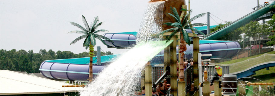
Next, let’s think about what a mathematical model looks like when we want to predict. For this one, let’s return to our discussion of the “tipping bucket/water park” system. Recall that here, we had a bucket held slightly off-center on an axle with water flowing into the bucket.

jungle-jims5

Periodically, the bucket would become unstable, tip, spill the contained water, and then return to the upright position and repeat. In this case, there is less mystery and less of a calling for an explanation. We can see that the system is mechanically driven, we have intuition about the changing stability, and we can see how it empties and resets. Here, what we want is to be able to predict the period of oscillation, given, for example, the physical properties of the system. That is, if we know the rate at which water flows into the bucket, the mass of the bucket, the volume and shape of the bucket, and the location of the axle, we’d like to be able to predict the interval of time in between tipping of the bucket. We’d like to be able to make this prediction for any given set of parameters for the bucket and perhaps be able to use this to design buckets that tip at different intervals. In this case, to accomplish this, we still make a hypothesis, namely that Newton’s Laws of Mechanics are governing the behavior of the system. But, it’s not really a hypothesis that we’re testing. Here, we have tremendous confidence in the hypothesis a priori. Rather, we’re accepting this hypothesis, mathematizing, and using the results of our analysis to make predictions about the world for systems we haven’t seen yet. Yes, we must still compare the results of our model to those of our observed system to validate. But here, the validation is more along the lines of making sure we did the mechanics and the mathematics correctly and less along the lines of testing the hypothesis that Newton’s Laws apply.

Finally, let’s think about the notion of using a mathematical model to control some real-world system. Let’s note that for both of the systems considered above, we can think about using the models we develop for control in some sense. In the case of Fairy Circles, once we’ve fully explained, we can look for parameters in our model that we can change in the real-world and that would produce different size circles, or perhaps, no circles at all. In the case of the tipping bucket, we can imagine changing the size of the bucket or the rate of the water flow and since we can predict how the period of oscillation will change, this gives us control over the system. These are certainly both examples of how we can use a mathematical model to control. But, I want to give you one other example that perhaps more clearly highlights this idea of using a mathematical model for control. Take a moment and watch this video clip:

This video shows the outcome of a project focused on implementing a classic feedback-control system for an “inverted pendulum.” The basic idea is simple and you can try it right now. Take a pencil and balance it by its point on your hand. You’ll likely almost automatically be able to move your hand to keep the pencil upright. The feedback you receive, visual and tactile, about the pencil’s position lets you rapidly adjust the motion of your hand to keep the pencil upright. Now, if you want to build a machine to do this, here’s where you need a mathematical model for control. Here, as with the tipping buckets, you would build a mathematical model based on the laws of mechanics. This model would tell you how your pendulum should move. But, in this model, you would build in an unspecified applied force to the system. Here, this unspecified part would be the motion of the base of the pendulum. By analyzing your model, you would then determine precisely how the base should move to maintain the upright position of the pendulum. This is then what you’d tell your machine to implement. That is, your mathematical model will tell you that if the pendulum has such and such a position and is moving and such and such a rate, you should move your cart in such a manner. That’s instructions that a machine can follow and you’ve now used a mathematical model to control a system in real time. In addition to the ways in which might use a model to control illustrated by the Fairy Circles and the tipping buckets, it’s useful to have this real-time, programmable sense in mind as well.

Hopefully these examples give you a clearer sense of the differences and similarities between building a mathematical model to explain, predict, or control. I encourage you to think through the goals of your models as you build them and as you first encounter a new modeling situation. In upcoming posts, I’ll work to demonstrate each of these three purposes in even more detail with further examples.

John
 

It’s winter in Delaware and while so far, it’s been a mild winter, today, we’re in the midst of a pretty good blizzard. Nonetheless, this past week I started planning my garden for the spring and thought some thoughts of spring might be nice to share today, especially for those of us on the east coast.

Last year was our first summer in our new house and so we just had a small vegetable garden in a flower bed along the back of the house. Now that I have a better sense of light and shadow, I’m ready to start planning out a small, but larger bed for this year. And, this past week, I got to thinking – Why not make it a smart garden?  That is, why not make it a garden that feeds me data about temperature, water content in the soil, hours of direct sunlight, and deer. Perhaps, I thought, I could make it self-watering and responsive to all that data. So, I enlisted the aid of my 14-year old son and we did some serious brainstorming about what we’d like in a smart garden.

We dreamed up a garden that not only would return us real-time data to our phones and would automatically water itself, but that also would detect and scare off predatory deer and other such annoying creatures. We talked about the garden regulating its own temperature and automatically picking ripe tomatoes, washing them, and putting them on the kitchen counter… then, we decided to start, well, more simply.

This led us to think about sensors, and measurement, and a little bit about the mathematical models that underlie sensing. I thought I’d share some of this thinking with you today.

We decided that the most important thing we needed to measure was the moisture level in the soil. Aside from weeding, which I don’t know how to automate, watering is the next most time consuming task, and one I think we can automate. While I generally don’t mind watering the garden, I do get distracted and forget sometimes, and that’s just plain not good for tomatoes. So, the question became – how do we know how much moisture there is in the soil?

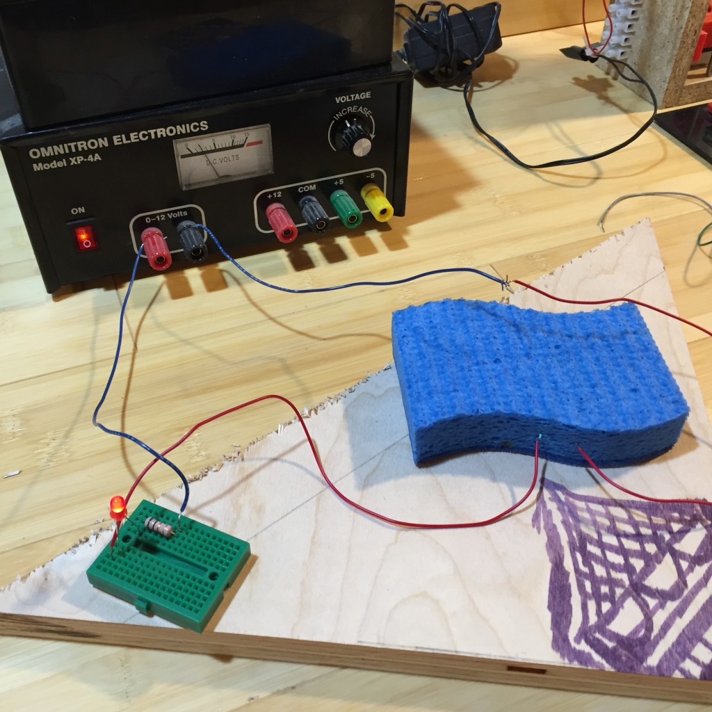
Let’s look first at the basic proof of concept demonstration that we rigged up, and then we’ll talk a little bit about indirect evidence and mathematical modeling. We used some wire, a sponge, a resistor, an LED, and a power supply, and built the following basic moisture sensor:

IMG_0242

The two red wires sticking out of the sponge have about 2 inches of insulation stripped off their ends. The wires aren’t connected, rather, these two bare ends are just stuck into the sponge. If the two wires were connected, the circuit would be complete, and the LED would light up. With the two wires held a distance apart in the sponge, the circuit won’t be complete at all when the sponge is fully dry, and will exhibit various levels of resistance depending on how wet the sponge is, for a wet sponge. This means the LED will light up with differing levels of brightness depending on how much water there is in the sponge. Voila! Moisture sensor.

Now, while this is pretty crude, it illustrates the basic idea behind lots and lots of different types of sensors. The idea is built on inference from indirect evidence. We can’t directly look and see how much water is in the sponge, so we set up something we can see that changes with how much water is in the sponge, and look at that instead. If you get this, you get the idea behind lots of sensors – if you can’t look at X, look at something that you can see that changes with X and infer how X much be changing.

Now, notice, this means that we need to know the functional relationship between the resistivity of the sponge and its moisture level. We’re measuring resistivity, in this case from the brightness of the LED, and we want to infer what that means about moisture levels. That is, whether or not we can make our sensor useful or not depends on whether or not we have a mathematical model of how the resistivity of this system changes with moisture. We can think about this model very simply as this functional relationship:

(1)   \begin{equation*} R = F(M) \end{equation*}

Here, R is the resistivity and M is the moisture content of the soil. In an ideal world, this would be a simple proportional relationship, we’d look-up or measure the constant of proportionality, and we’d have a simple and useful way to determine moisture. But, of course, as in all things we want to model in the real world, things aren’t quite as simple as the ideal case! Perhaps the biggest complicating factor is that soil resistivity varies with other things that are likely to be changing in our system. In particular, it varies with temperature and with the ionic content of the water. As in any modeling problem, the question then become whether or not these impact the functional relationship we’re after to a degree that impacts this relationship in a meaningful way. Here, it may be safe to assume that ionic content doesn’t vary much over the life of the garden and we can ignore it. Temperature, on the other hand, does vary a lot, and it turns out that on the scale on which we’re trying to measure this functional relationship, the variation of temperature has a significant effect on F. So, we really need to be thinking about a mathematical model of the form:

(2)   \begin{equation*} R = F(M,T) \end{equation*}

Here, T is temperature. Now, there are two paths one could take to obtain F and these nicely correlate with the notion of descriptive and analytic models that we’ve explored before in this space. In this context, a descriptive model of the situation is often called an empirical model. You can imagine that we could obtain F by designing a set of experiments. For example, we could take a sample of soil and thoroughly dry it out in the oven, let it come to some known temperature, and then measure R. We then add known quantities of water to this known volume of soil and measure R along the way. We then repeat this for a bunch of different temperatures, T. In this way, we build up a data set to which we can fit a curve that becomes our model, F. In situations like this, and for moisture sensors, this is the general approach. An alternative, analytic path, would involve computing the resistance from first principles. That would mean we’d need a good model for the soil composition as a function of space, the resistivity of each of the constituents of the soil, the flow of water through the soil, and how all of these things respond to temperature. In this case, the complexity of such a model and the work involved in the analysis isn’t likely to be worth the payoff. It might be interesting and I’d bet that someone, somewhere has done it, but if all we’re interested in is calibrating and using our sensor, I’d go with the empirical model here.

Now, this train of thought got me to thinking about a lot of the STEM activities I’ve seen used in K-12 and how often, these involve measurement of one form or another. I’d like to encourage you, when you think about such activities, to think about the measuring you’re doing a little more deeply than you might be used to. For those very many cases where you’re doing some sort of “can’t see X, so I’ll measure something I can see that varies with X,” it’s probably worth taking a moment and having your students think through the mathematical model you’re relying upon to make that work. Hopefully this will give your students a deeper appreciation of another aspect of the interplay between S, T, E, and M. And, if your students get real ambitious and want to come design and build my new smart garden, let me know. Always open to help!

John

Over the last several months, we’ve explored mathematical modeling from a variety of perspectives here in this space. We’ve talked about the CCSSM, the modeling cycle, thought tools used by modelers, and we’ve explored a variety of examples, all with the goal of trying to understand how mathematical modelers think and how we might best train our students in the art of mathematical modeling.

One thing we have not done is follow the path of a typical course in mathematical modeling. Today, I want to talk a bit about what such courses look like, and where we might benefit from typical paths and why we might want to deviate from typical paths. Until recently, at least in the United States, mathematical modeling courses have largely been restricted to higher education. They’ve been taught primarily at the advanced undergraduate level and the graduate level. There are exceptions and there have been efforts to teach such courses at the introductory undergraduate level, but it’s reasonable to claim that the majority of the effort around teaching mathematical modeling has primarily occurred at the upper undergraduate and graduate levels.

This means that the majority of textbooks focusing on mathematical modeling are also aimed at the upper undergraduate and graduate levels. If you search for “mathematical modeling” on Amazon, you’ll, in fact, find several thousand books along these lines. Some are more specialized, some are less specialized, but generically, they are aimed at this advanced audience. If you examine the most popular of these, the ones that focus on “mathematical modeling” rather than “mathematical modeling in X,” you’ll find they all follow a typical pattern and that this pattern is reflected in course syllabi at institutions across the country. Roughly speaking the pattern is one where the texts are organized by mathematical topic first, and application areas within those topics. That is, you’ll see them divided into chapters with titles like “Modeling with difference equations,” “Modeling with ordinary differential equations,” “Modeling with partial differential equations,” and so on. Within each chapter, the authors will introduce an application area, and then show the reader a bunch of models developed in that application area using the mathematics of the chapter heading.

The philosophy behind this approach is one of “modeling can’t be taught, but it can be caught.” That is, authors and instructors largely assume that if they show students enough examples of mathematical models, they’ll eventually catch on and know how to model. I freely admit, that I too was a member of this camp for a long time. After all, it had worked for me! But, in teaching mathematical modeling over the last twenty some-odd years, and especially as I’ve had the opportunity to work more closely with the K-12 community, I found myself growing increasingly frustrated and disillusioned with this approach. In the large majority of cases, it became apparent to me that while a handful of students did “catch it,” the vast majority did not. They could perhaps use models they’d seen before, and engage in somewhat trivial extensions of such models, but when faced with a new situation, they were lost. They hadn’t, by and large, learned how to actually model. They hadn’t become modelers.

I gradually realized that I don’t agree with the “can’t be taught, but can be caught” philosophy and many of the blog posts here have been inspired by my personal change in perspective on this issue. I believe that we can, in fact, deconstruct and understand the process that constitutes mathematical modeling, articulate this process more clearly for our students, design activities to engage students in essential competencies that comprise this process, and end up teaching a lot more students how to actually model. My colleague, Rachel Levy at Harvey Mudd, says that what we’ve been doing for a very long time is teaching “model appreciation” rather than teaching the art of mathematical modeling. I think there is a lot of wisdom in that statement and that we can make this shift, at all levels, from teaching model appreciation to teaching the art of mathematical modeling. As I’ve had the chance to explore the mathematics education literature on this topic, especially the international literature, I’ve learned that there has been progress made in this regard and I’ve worked to incorporate the best of these ideas into my own teaching and try and share some of them here.

But, in the back of my head, there is also this whole “baby with the bathwater” thought that’s been nagging me for a long time. In an earlier blog post we explored the notion of “thought tools.” These are those ways of thinking that are often widely applicable and are characteristically wielded by those who engage at a high level in a particular practice. We talked a bit about some of the thought tools wielded by mathematical modelers. This thought tool perspective pushed me into doing a lot of meta-thinking – trying to observe my own thought processes as a mathematical modeler and compare them with those of students just learning the art.

One thought tool that I find myself wielding frequently and have observed other mathematical modelers utilize as well is “analogical thinking.” That is, when faced with some unfamiliar modeling situation, a modeler will often start by arguing “well, this situation is kind of like situation X, so perhaps we can proceed as follows…” They have, in their head, a repository of modeling approaches for a wide variety of problems. They rely on the miraculous fact that mathematics and mathematical approaches to applied problems are often wonderfully generalizable, and so develop solutions to new problems relying at first on what they’ve seen work before. The uniqueness of each situation requires adaptation and creativity, but they can often grasp a ready starting point from which progress can be made.

That brings us right back to model appreciation, because after all, where did they get this broad experience with various modeling approaches? Well, they’ve looked at and worked through lots of models built by others to tackle lots of different situations. Seems they caught something useful somewhere along the line. The seemingly presents us with a dilemma. The vast majority of students don’t catch modeling by the model appreciation approach, but the experience gained via model appreciation seems essential to be a good modeler. I don’t think this actually a dilemma. I think that we should conclude that we need to engage students in both some model appreciation and some deconstruction and practice of the art and the process of thinking like a mathematical modeler. I believe, and can claim from my own personal experience, that this dual-approach, is a more successful approach.

So, as you think through and work to incorporate mathematical modeling into your classroom, I suggest you keep this dual approach in mind. Spend time giving students the opportunity to practice modeling on new and fresh situations, help them understand the process and the practice, pay attention to developing the thought tools they’ll need and the competencies they must master, but, from time to time, don’t be afraid to engage in a little model appreciation and help your students start to build their own “model repositories” in their heads.

John