In addition to having the opportunity to work with mathematics teachers implementing mathematical modeling in their classrooms, I also often have the opportunity to work with groups of teachers from across math and science who are trying to implement “STEM” ideas in their teaching or in extra-curricular activities. This has given me the chance to think through the notion of STEM and in particular, to think carefully about the role of mathematics and mathematical modeling in the K-12 teaching of STEM.

One of the most useful articles I’ve found for understanding the “big picture” and history of “STEM” is an article called “Evolution of STEM in the United States” by Professor Emeritus William E. Dugger, Jr., of Virginia Tech. Dugger carefully defines each of the letters in the acronym “STEM.” He offers that:

S – Science, which deals with and seeks the understanding of the natural world, is the underpinning of technology.

T – Technology, on the other hand, is the modification of the natural world to meet human wants and needs.

E – Engineering is the profession in which a knowledge of the mathematical and natural sciences gained by study, experience, and practice is applied with judgement to develop ways to utilize economically the materials and forces of nature for the benefit of mankind.

M – Mathematics is the science of patterns and relationships.

Within these four definitions one already begins to see the interrelated nature of these areas and their dependence upon one another. Readers of this blog will also note his characterization of mathematics as the science of pattern and relationships; again, this way of thinking about mathematics illuminates the deep connections and utility of mathematics for S,T, and E.

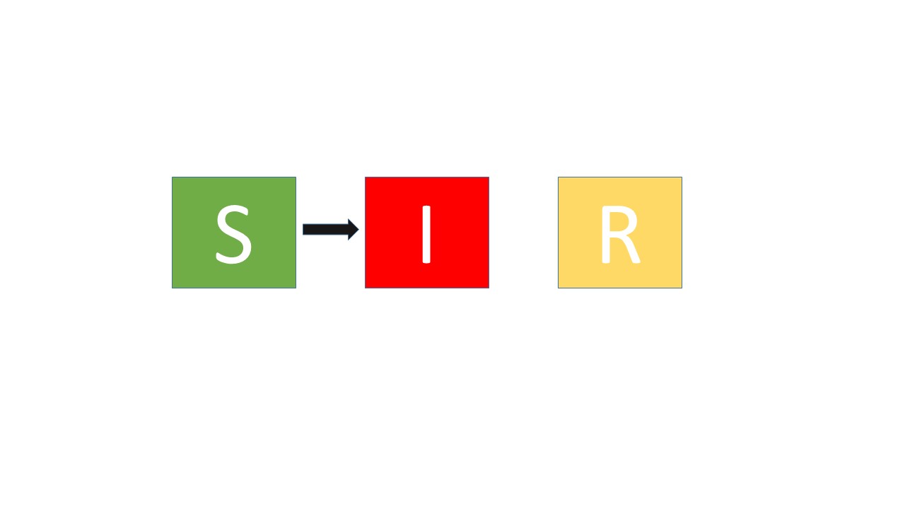
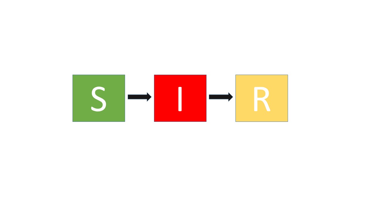
Dugger also offers several models of the way STEM is, or can be taught. The first of these is the “silo model,” where we view STEM as “S-T-E-M,” with each discipline being fully distinct and independent and taught with no integration among the four. The second is similar, retaining the silo nature, but emphasizing some disciplines more than others. Dugger labels this one as “S-t-e-M,” with the upper and lower case indicating levels of emphasis. A third model occurs when one of the four disciplines is integrated into the other three. The most common is when the “E” is integrated into the rest. Dugger denotes this as “E -> S,T,M.” Here, the S,T, and, M, remain in silos, but the E is integrated into each. Dugger’s final model is the fully integrated approach, where each of the four are integrated into one another. This, in effect, has us view STEM as a “meta-discipline” and this kind of integration can be simply denoted as “STEM.”

When I work with STEM councils or groups working to create STEM opportunities for students, it’s this last model that I emphasize. For me, this “meta-discipline” or integrated approach is what’s necessary if our students are going to be able to work effectively in the scientific community of today and contribute to the solution of our most pressing challenges. Nature recently released a special issue on interdisciplinarity with the subtitle “Why scientists must work together to save the world.” This is just one more voice in the chorus of voices calling out for bridges between the myriad array of disciplines created as a result of fifty years of hyper-specialization. Helping students experience an interdisciplinary perspective and be prepared to work in interdisciplinary teams seems like a worthwhile goal for those working to create STEM opportunities for students. Note that this doesn’t diminish the importance of the disciplines or obviate the need for deep content knowledge, but rather, creates opportunities to bring that content knowledge to bear on problems that can’t be solved by working solely within disciplinary boundaries.

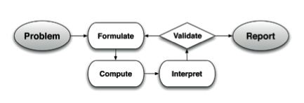
This, of course, bring up the challenge of actually doing this in practice in K-12. What does a good STEM activity actually look like? The risk is that we create activities where students do a little “S” and a little “T” and then a little “E” and then we throw in a little “M” and we’re back to the “S-T-E-M” model rather than the “STEM” model. To help people think about “STEM” vs. “S-T-E-M” and designing good STEM activities, I encourage them to think in terms of the three central practices of STEM. In shorthand, we can think of these three practices as theory, experiment, and design. You may be more comfortable thinking of these in terms of cycles that you’ll find in the NGSS and CCSSM, namely, the mathematical modeling cycle, the engineering design cycle, and the scientific method. One way to picture the relationship among these cycles or among the practices of theory, experiment, and design is:

IMG_0225

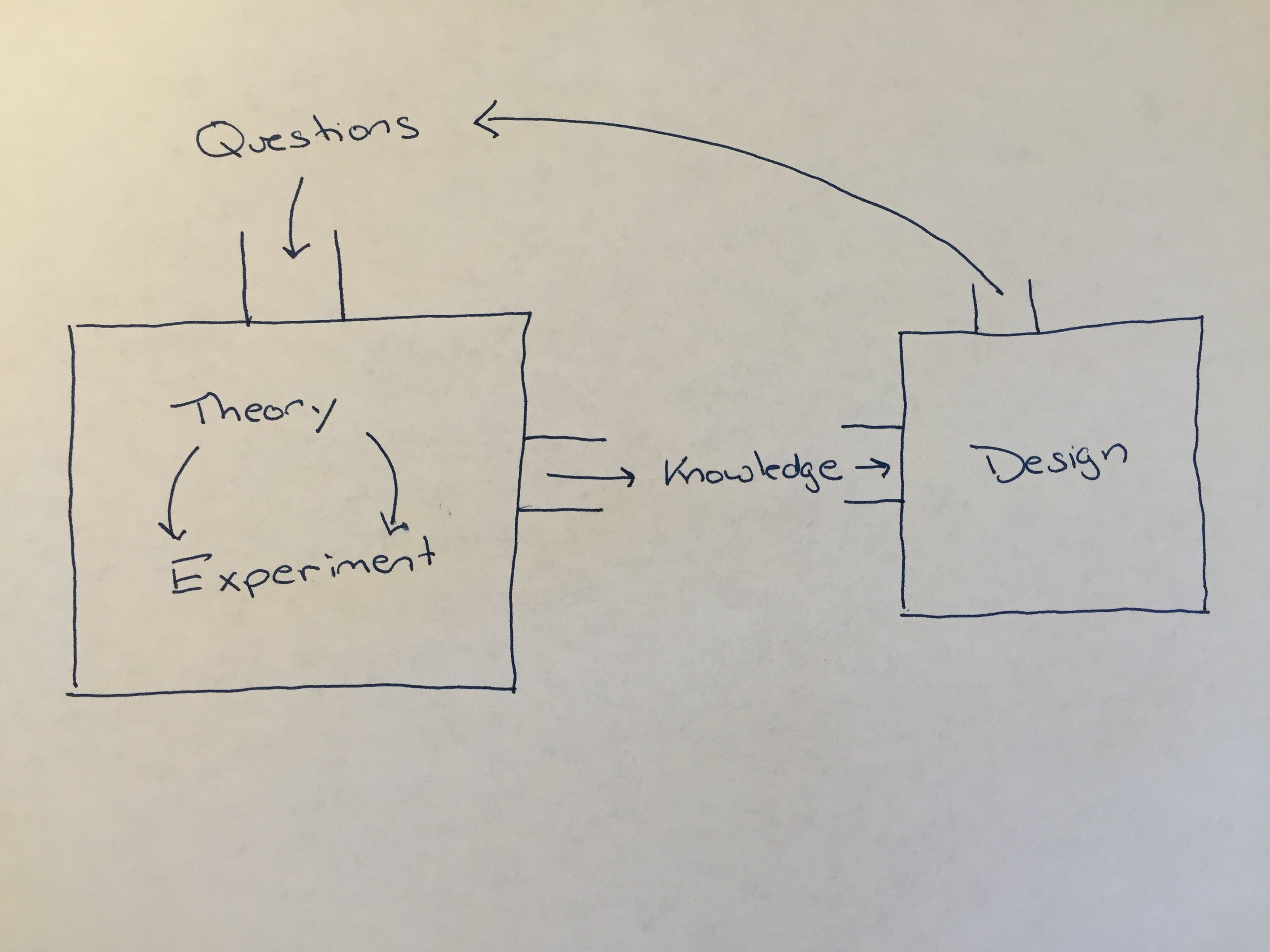
That is, we have questions about the real-world. We use the tools of science to find explanations and build the ability to make predictions. These tools of theory and experiment, or modeling and experiment, generate knowledge about the world. We take this knowledge and use that to design technology that lets us control and modify our world. Doing so often creates new questions that we then again turn to theory and experiment to explore, and so on.

A good STEM activity engages students in this sort of interplay of the central practices. The starting point can be anywhere in the diagram but shouldn’t stay confined to a particular box. In practice, it’s often easiest and most easily engaging to start in the “design” space, that is, to start with what we might think of as an engineering challenge. But, a really good engineering challenge will have students asking questions that they need to turn to theory and experiment to answer. They’ll get a deep sense for how science informs engineering and how engineering challenges lead to interesting scientific questions. And, along the way they’ll engage in mathematical modeling, engineering design, and the practice of science.

Now, this is still all rather abstract! Next time, I’ll make this very concrete and we’ll explore a particular STEM challenge and see exactly how the interplay pictured above might look in an activity appropriate for K-12 students. Till next time!

John


Last weekend, I had the chance to spend the day in NYC with my daughter. While most of our day was taken up with a college recruiting event, I couldn’t resist taking her to visit one of my favorite bookstores in the world, the Strand Bookstore at the corner of 12th and Broadway. Housing 18 miles of books, both new and used, the Strand calls out for serendipitous rather than targeted browsing. I’ve never been disappointed and never walked out with anything I would have anticipated in advance.

Last week, I stumbled upon (and bought, couldn’t resist), an out-of-print book called “The Way Things Work.” It’s actually a two-volume set, billed as “An illustrated encyclopedia of technology.” What made it irresistible to me was its structure and the fact that it was about one thousand pages of cool models. Every pair of pages consists of a brief paragraph of text describing a particular piece of technology, and on the facing page are pictures, illustrations, models. I scanned a few pages so I could share them here. Here’s the one on elevators:

SDeanCopier15110911070_0001

And, here’s one on speakers:

SDeanCopier15110911060_0001

I wanted to share these pictures, these models, because they reminded me how important such models are, not only in communicating understanding, but in the mathematical modeling process. When we think about the mathematical modeling cycle and the often daunting “Formulate” phase, we often leap directly to thinking about formulating in terms of mathematics. But, that’s not what you’ll find most modelers actually doing in practice. That is, they don’t leap from “Problem” to writing down well-formulated mathematical equations describing a system. Instead, if you watch modelers at work, they’re likely to start by drawing pictures. Lots of pictures. Lots and lots of pictures. The reality is that most of us don’t think in terms of equations. We think in terms of pictures and stories and the process of sketching out a picture of the system we’re trying to understand and telling ourselves the story of the process that’s happening in the system is how we first develop understanding. As we’re sketching and talking through what we believe is happening, we’re simplifying and making approximations. We’re leaving things out of our pictures and putting other things in. We’re developing a conceptual model of what we believe is going on. We’re starting to introduce notation and often, geometry. We’re making guesses and conjectures about what’s driving what we’re observing. It’s usually only then, only after we’ve gained some simplified hold over the system, that we start to translate and turn that understanding into mathematics.

Last week, I was also reminded of the importance of pictures and story in the modeling process by a fellow named Anton (Tony) Weisstein. Tony is a mathematical biologist and teaches at Truman State University in Missouri. Much of his work focuses on developing innovative curriculum materials for the teaching and learning of mathematical biology, and much of this focuses on finding ways to teach the art of mathematical modeling to biology students. Tony was visiting the University of Delaware and I had the chance to attend a workshop he conducted on his approach.

The example Tony used was the modeling of the spread of infectious disease. In mathematical biology, there is an incredibly widely used and wildly successful modeling approach to such problems known as the “S-I-R” model or the “S-I-R” class of models. When introducing his students to these models, Tony starts with a discussion of infectious disease and guides his students to slowly sketch a conceptual model of how they envision such diseases being transmitted. He draws his first sketch like this:

SIR1

The discussion to this point has been about the types of individuals that could be in the population of interest. Tony’s steered the class to identify three key categories within that group. The first, “Suceptible” is represented by the box labeled “S.” This is the group of people who could get the disease. The second, “Infected” is represented by the box labeled “I.” This is the group of people who have the disease. The third, “Removed” is represented by the box labeled “R.” This is the group who has perhaps died, recovered, or otherwise been permanently removed from the population of those who could get or have the disease. Here, Tony stresses something important – he says “let’s start with the simplest possible scenario, we can always complicate things later.” He encourages students to remember or write down all those complications so that they can return and think them through later. Next, Tony focuses the discussion on the process. How can  individuals move from one box to another? When the class says “Someone who is susceptible can get infected,” Tony modifies the picture to include this idea:

SIR2

Further discussion leads to the idea that someone who is in “I” can move to “R” and another modification of the picture:

SIR3

In this way, Tony elicits a complete conceptual model of the situation from the students before ever thinking in mathematical terms. His pictures are, to me, of the same character as the pictures from “The Way Things Work” and very much like the sketches and diagrams you’ll happen upon if you catch a mathematical modeler at work.

I’d encourage you, as you work with your students, to encourage drawing and sketching and storytelling as you and they discuss the phenomenon you’re trying to model. Building these conceptual models and clarifying your thinking by sketching and explaining the process makes your work in the “Formulate” box of the modeling cycle much easier and much more fun.

John


How many piano tuners are there in the United States? How many golf balls would it take to circle the earth at the equator?  How many ping-pong balls would fit in the Superdome?

We’re often asked if questions like these are the basis for a good modeling exercise or if a student answering questions like these is engaged in mathematical modeling. My general answer? “Maybe” or, “It depends.” Today, I’d like to explore this question a little bit and think through how such questions can be a way to engage students in the art of mathematical modeling and what it takes to investigate one of these questions from a modeling point of view.

Problems like these are often referred to as “Fermi Problems” after the Italian physicist and Nobel Laureate, Enrico Fermi. Fermi was known for his ability to make quick, remarkably good, estimates to answer questions like these. Sometimes we refer to the calculations involved as being “back-of-the-envelope,” indicating a sort of rough order-of-magnitude estimation procedure for obtaining estimates. Sometimes, these types of questions become interview questions at firms like Google, purportedly to test a candidate’s ability to think quickly and reason quantitatively. There is no doubt that this skill of estimation is an important part of what we mean by “quantitative reasoning,” and there is no doubt that quantitative reasoning is an important skill for mathematical modeling. But, is an investigation of a Fermi Problem the same thing as doing mathematical modeling?

To answer this question, let’s take a particular Fermi Problem and think about two different investigations, one which stays pretty clearly embedded in the realm of quantitative reasoning and a second which shows how we might develop such a problem and push our students to genuinely take a modeling perspective on the question. Since ping-pong balls are always fun and generally familiar, lets take up the question – how many ping-pong balls would fit in the Superdome?

Now, one way to think about answering this question would be to simply take the volume of the Superdome and divide by the volume of a ping-pong ball. In pre-Google Fermi days, we’d need to figure out how to estimate both of these quantities, but now we can get good estimates of these two volumes with just a few keystrokes. Since the first numbers that Google gave me were in cubic feet, I’ll work in these units. I found:

Volume of Superdome \approx 130,000,000 ft^3

Volume of a ping-pong ball \approx \frac{4}{1750} ft^3

Dividing, I obtain:

Number of ping-pong balls in Superdome \approx 56,875,000,000

And, I’m done. Generally, with most Fermi problems, one says “wow, that’s a lot of ping-pong balls,” and the discussion ends.

Now, let’s think about what we just did in the context of the modeling cycle.

160518_3

We started with “Problem,” i.e., how many ping-pong balls would fit in the Superdome? We can argue that we moved to “Formulate” when we said “divide the two volumes,” but that already feels a little forced.  We could argue that we went through the “Compute” stage and perhaps even the “Interpret” stage when we took our final number and said “almost 57 billion ping-pong balls” as an answer, but that feels even more forced.  And, what about that “Validate” part? What about comparing back to the real-world? What about the whole cyclic nature of mathematical modeling? I’d argue that if this is the type of discussion around a Fermi Problem, then, no you’re not really doing mathematical modeling. That’s not to say that you’re not doing something valuable, but at the same time, you’re not really involving your students in mathematical modeling and you’re not really training them in thinking like a mathematical modeler.

So, the question becomes – what would an investigation of this problem look like if we really wanted to use it as a way of having students experience the art of mathematical modeling in a more genuine manner?

Consider an alternate approach. We begin, as before, by reasoning about volumes. This time, perhaps, we introduce a little notation, and think about the question a little more generally. For example, we might say the number of ping-pong balls, N, that fits in a given space is a function of the volume of the space, V_s, and the volume of a ball, V_b. That is,

N = N(V_s, V_b)

Now, our initial model of this dependence is as before:

N = \frac{V_s}{V_b}

Why is this different than what we did before? Well, in one way, it’s not. We could repeat the steps from before, substituting in the same estimates as above for V_b and V_s and obtain, of course, the same answer. But, expressed this way, we can also more easily think about this functional dependence that so often lies at the heart of mathematical modeling. If I increase the volume of the ball, N decreases in an inversely proportional way. If I increase the volume of the space, N increases in a directly proportional way. This hypothesized functional relationship makes intuitive sense. Written this way, I can also easily think about model validation. While I can’t afford fifty-six billion ping-pong balls nor get away with filling the Superdome with ping-pong balls, I can fill a shoe box. I can actually do that experiment, fully, and compare it to my model’s prediction. This will give me a sense of whether or not my model is realistic and believable. And, if I do that, I’d find that my model overestimates the number of balls I could fit in a shoe box (or any box) by about 25%. This would likely lead me to realize that ping-pong balls don’t pack together without gaps, and I’d be driven around the modeling cycle, and inclined to modify my model, perhaps by including a space filling scale factor:

N = c \frac{V_s}{V_b}

We could now think about and explore how this scale factor, c, depends on the shape of the object filling this space. That is, c takes one value for a sphere, but a very different value for a cube. We could even now think about our modeling efforts from both a descriptive and analytic view point. From a descriptive viewpoint, we could fill different sized boxes with ping-pong balls, gather data, and fit a curve to this data. How does this curve match with our proposed analytic model above? When we think about the analytic model we’ve proposed, we could think about the underlying principles about the real-world we’ve had to posit in order for this model to make sense. For example, we’re relying on a “ping-pong ball exclusion principle” that says no two ping-pong balls can occupy the same space at the same time. We’re assuming that the Superdome is empty and ignoring all those bleachers already filling the space. We’re also assuming the ping-pong balls don’t deform under the weight of those above them. Would this really hold true in the Superdome?

If we returned to the modeling cycle and tested our thinking against the cycle with this approach to the problem, I think we’d be able to convincingly argue that we’re genuinely making use of an iterative modeling approach this time around. Now, that’s kind of interesting – after all, in both cases we’re ostensibly solving the same problem. How can it be that in one case we’re “modeling” and in the other, we’re not? The key is that modeling is not just about your choice of problem. Modeling is both about the choice of problem AND the approach you take to solve that problem. Remember we build mathematical models to explain and predict. In the second approach to our ping-pong ball problem, we’re not seeking a number or an estimate as much as we’re seeking insight and understanding.

If we take the time to do Fermi Problems in the second way described above, and carefully pick the types of Fermi problems we think about, I do think that the investigation of at least some such problems can provide a valuable way to introduce students to the process of mathematical modeling. They have the advantage of being easily understood as problems and of relying on extra-mathematical knowledge that’s likely to be in the toolbox of even young students. I encourage you to attempt some Fermi Problems with your students and try them from a modeling perspective.

John


I’m fortunate in that my current position at the University of Delaware gives me the flexibility and opportunity to fairly regularly spend time in Delaware schools talking with and working with Delaware teachers. It’s especially fun to speak with teachers who are just starting to incorporate the practice of mathematical modeling into their classrooms. Today, I’d like to talk about a fairly typical dilemma or stumbling block that these teachers face and share some ideas for how to get past common sticking points.

The common dilemma is this – many teachers find a great real-world problem for their students, find a nice real-world data set for them to work with, and get their students genuinely engaged in investigating this problem. The students then grab the first tool in their toolbox, i.e. curve fitting or regression, fit a nice curve to the data, make a nice plot, and then say “Now what?” That is, the teachers we have worked with are very comfortable carrying out descriptive modeling and very comfortable working in the “compute” and perhaps “interpret” or “validate” boxes of the CCSSM modeling cycle, but then find themselves at a loss for what to do next. These teachers generally sense that there’s something missing, but then can’t quite find their way forward with a next step.

I asked Michelle about this common phenomena and asked for her perspective as a former high school teacher in particular. Here’s what she had to say:

This dilemma resonates with me. Because I did not take any coursework in mathematical modeling as a secondary education major (an issue which is a national problem according to this article by Newton et al. (2014), I did not have a good sense of what mathematical modeling was really about. My notions of mathematical modeling were largely formed by my engagement with curriculum materials. This is problematic because, as pointed out by Meyer (2015), many textbook exercises labeled as “modeling” tasks do not authentically engage students in all aspects of the mathematical modeling cycle. It was not until graphing calculators, and subsequently regression problems, became an important part of school mathematics that I really had any opportunities to engage in any form of modeling. At the time when it was introduced into school mathematics, I either had to teach it to myself or attend professional development workshops to learn about calculating these simple descriptive models. However, unlike the teachers described above, I thought I was done once the line of best fit was calculated, and I verified a “good” r-value. It is promising to see that these teachers are aware that there should be more to modeling than this. 

It’s encouraging to know that there has already been a shift in how teachers are thinking about mathematical modeling and that at least in my experience in Delaware, are trying to think beyond curve fitting. But what should a teacher who is faced with this dilemma do? How do you get past that feeling of “Now what?” or take your modeling beyond simple curve fitting? Based on my observations, I want to offer two pieces of advice or two strategies you might follow when faced with this dilemma.

Strategy #1 – Go back to the beginning

It seems to me that a common reason why this dilemma occurs at all is because not enough attention was paid up front to the “Problem” phase of the modeling process. It’s important to remember that what you are doing is trying to answer a question and that question is not a mathematical question! That is, being able to fit a curve to data is not the point of the exercise. Rather, your students should clearly have in mind the real-world problem that you’re trying to solve or the real-world question that you are trying to answer. It’s this question that drives you around the modeling cycle and this question that you should be returning to once you’ve done something like fit a curve to a data set. So, when faced with “Now what?” one answer should always be “What question were we trying to answer to begin with?” Bringing the focus back to your core question is one way to move the conversation forward.

Strategy #2 – Validate and critique the model

What do you do when your students say “we’ve fit this curve to our data, we have a good r-value, and hence we can now predict that in the future there will be X of Y”? That is, what do you do when they’ve done regression and think they now have entirely answered their real-world question? Here’s where you have an opportunity to push the conversation forward by validating and critiquing the model. I’d ask students questions like “how much confidence do you have in your prediction?” or “do you have any reason to believe that the trend you’ve sketched out will continue indefinitely?” Most curves obtained by curve fitting, when pushed beyond the range of data where they were obtained will lead to results that are genuinely open to question. This might be because we have no real reason to expect such trends to continue or it might be because we have no real reason to expect such trends to even exist, as we saw in The Shrinking Mississippi. Opening a conversation like this, allows you to help your students understand the limitations of all models, especially those that are purely descriptive models. This creates an opportunity to return to the start and push your students’ thinking toward analytic models built on a more fundamental understanding of what it is that they are exploring.

It’s important to remember both that mathematical modeling is a cyclic process and that what drives one around the cycle is the attempt to answer a real-world question. When you’ve built a model and are faced with the “Now what?” question, keep the goal in mind, be critical of the models you’ve built, and you’ll find ways to help you and your students be able to say “Oh, that’s what’s next!”

John