Mathematics is the science of pattern and when we are doing mathematical modeling, we’re extending or tying the investigation of pattern explicitly to patterns in the real world. These might not be clear, simple, spatial patterns like those that usually occur to us when we hear the word “pattern.” They might be patterns in time, or patterns in some observed data set. But, sometimes, like in the case of the so-called “Fairy circles of Namibia,” they just might be clear, simple to observe, spatial patterns in nature.

Recently, these fairy circles were back in the news due to an article about their origin that appeared in Ecography. Science News published a short piece on fairy circles, covering a bit of the history of the search for an explanation, and an update on recent thinking. Their article, titled “What fairy circles can teach us about science,” got me to wondering what fairy circles might teach us about mathematical modeling.

So, today, I’d like to explore fairy circles, how we might approach this phenomena as a mathematical modeler, and hopefully demonstrate how a question still open to modern science can be accessible to investigation in the high school math classroom. I want to do this in some detail, so, fair warning, this will be a multi-post sort of investigation.

Let’s start by just looking at fairy circles. Following is a picture of the phenomena from an article by CNN addressing the topic. You can find plenty of such pictures with a simple Google of “fairy circle Namibia.”
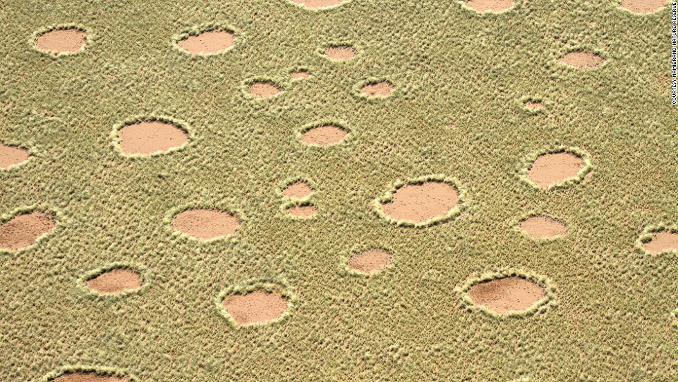
Fairy circles

Fairy circles

I think the picture makes the basic phenomena quite clear. You’re looking at a section of desert, where the green is plant life, and the open circles are simply bare spots, devoid of plants. These circles dot the landscape of a 2000 km long strip of desert, each circle somewhere between 5 m and 10 m in diameter, and the circles grow, shrink, disappear, and reappear in time. The question of course is – why the heck are there bare circles?

They get their name of “fairy circles” from the explanation that they are created by gods, spirits, or fairies. The image of thousands of fairies deciding to take a break, landing in the desert, and creating a nice little circular clearing for themselves is an appealing one. Over time however, various alternative theories have been proposed. These include toxic soil, termites, and radioactivity. They also include the idea that these patches are the result of self-organization, and that they occur naturally as the result of competition for scarce water resources between plants in the desert. This is the hypothesis that I’d like to investigate here.

The idea of self-organized pattern formation is generally attributed to Alan Turing. Yes, the same guy that cracked the Enigma machine, invented the computer, and who was so ably portrayed by Benedict Cumberbatch in The Imitation Game.  (If you haven’t seen it, great movie!) Among other things, Turing was interested in patterns that occurred in living systems. That is, things like the stripes on a zebra or the spots on leopard. In a paper called “The Chemical Basis of Morphogenesis,” he showed how the processes of chemical reaction and diffusion could combine, under the right circumstances, to create sharp spatial patterning. This early paper triggered years of investigations by scientists into pattern formation based on this mechanism and related mechanisms. The mathematician Jim Murray captured a huge amount of this work in his excellent book “Mathematical Biology.” Now, the first point I want to make is that Turing’s investigation, and most of the subsequent investigations into pattern formation have been carried out via mathematical modeling. This area of pattern formation in living systems, given that mathematics is the science of pattern, has been an incredibly ripe and fruitful area for the mathematical modeler.

So, back to Namibia. When a mathematical modeler sees a spatial pattern, like fairy circles, they think “self-organization.” Now, what does that mean? Well, in general, that means they are inclined to look for some underlying physical mechanism, usually some form of competition between effects or between things, and then to see if this mechanism can indeed drive the system toward forming a pattern spontaneously. From the work of Turing and all those who followed him, they know that this isn’t unlikely. In fact, they know that lots of spatial patterns in nature, from the stripes on a zebra to the patterns created by the growth of bacteria in a Petri dish can be understood in this way. So, seeing fairy circles and hearing the hypothesis of self-organization as an explanation is a perfectly reasonable thing for the modeler. Their job is to then see if they can test this hypothesis by mathematizing the proposed underlying physical mechanism, and then analyzing the mathematical model to determine if there are conditions under which spatial patterns will indeed form. In this way, they are testing the hypothesis that the proposed physical mechanism can lead to the patterns observed. If their model can be shown to not lead to pattern formation, then they’ve ruled out the proposed mechanism as the sole cause of the patterns. If it can be shown to lead to pattern formation, then the mathematical conditions under which this happens can be checked against the real world, either strengthening the case for the proposed mechanism or suggesting refinements to the model.

This is the approach taken by Getzin et. al. in the Ecography paper mentioned above. They’ve built a mathematical model that “supports the hypothesis that fairy circles are self-organized vegetation patterns that emerge from positive biomass-water feedbacks involving water transport by extended root systems and soil-water diffusion.” Okay, that’s a mouthful, and their mathematical model is pretty darn sophisticated. It’s a system of non-linear partial integro-differential equations for… well, it’s complicated. So, why would I claim this is a problem appropriate for the high school classroom?

Ah! That’s a pretty good cliff-hanger, so let’s break here for today and pick up next time with this question. In the meantime, perhaps you might think about how your students might think about this problem. That is, suppose you told them about fairy circles and that competition between plants was a proposed mechanism behind the patterns. How might they investigate this through mathematical modeling? How might you? Till next time…

John


Back in “Curiosity, golf math, and another tool for your classroom,” we explored the high-speed video capabilities of the iPhone 6 and talked about how we might use this tool to develop interesting mathematical modeling problems. High speed photography, like that of the iPhone, lets us “see fast.” That is, we can use that tool to see things that happen more quickly than we can ordinarily perceive.

Well, the iPhone (and iPad, and iPod touch) lets us go in the other direction as well. We can take advantage of the time-lapse photography mode and see slow. That is, we can capture things that happen so slowly that the change is not within our typical perception of events.

One of my favorite summertime “seeing slow” things to do is to get up early and watch the sunrise over the ocean. This year, I was fortunate to have a chance to spend a few days in Cape May, NJ, with beautiful weather, and plenty of opportunities to watch the sunrise. I decided to take this opportunity to explore the time-lapse capabilities of the iPhone and to think a bit about how we might use time-lapse video to create mathematical modeling opportunities in the classroom. Here’s one video I took that spans about 30 minutes of real-time and 27 seconds of “time-lapse” time:

In time-lapse mode, the iPhone dynamically chooses the frames per second captured for a time-lapse video, with the frame rate dependent on the total length of the video. For a video that is between 20 and 40 minutes long, like this one, it takes one frame per two seconds and then speeds up the playback time to 60 times normal speed. If the normal playback speed in 30 frames per second, it is now playing the equivalent of 1800 frames per second, so we see 60 seconds of real time for every one second of video. That’s what you are watching in this video.

Now, watching the sun rise like this got me to wondering – how many students have actually seen the sun rise? How many have thought about how “brightness” changes as we go from dark to light? If I asked my students to plot “brightness” versus time as we transitioned from before sunrise to after, what would their plots look like? If you get a chance to ask your students this question, please share their thinking!

In the meantime, let’s see what we can actually learn about how brightness changes using our time-lapse video of a real sunrise. Along the way, we’ll learn a little bit about image processing, and pick up a few more tools for you and your students to use during your investigations.

We’ve already seen how easy it is to collect data using an iPhone or similar device in the form of video. The problem is that video isn’t the most convenient format to use when what we want is numerical data. It is generally much easier to extract numerical data from a still photo. So, the first thing we need to do is extract individual frames from our video. Fortunately, this is pretty easy and you can do the job with a free piece of software called VLC Media Player. It’s ad free, easy to use, and available for just about any operating system you choose. You can easily find instructions as to how to do the frame extraction from video, so I’ll let you read about that elsewhere. This web page is a good start.

The more interesting question is what to do with the still photographs once you have them. This is where we need to do a little image processing and to do that it’s helpful if we know how to do a little coding. In fact, knowing how to do a little coding is pretty much an essential skill for the mathematical modeler. At the very least, being able to do a little coding vastly extends the range of what you can do with your mathematical models and for models that are mathematically complex, being able to code and obtain a numerical solution to your problem is often the only path forward. So, I’d advocate having your students learn to tap into the power of computing every chance you get! There are an incredible number of programming languages available now, many designed for the first time coder and for very young students, so this isn’t nearly as challenging as it was even twenty years ago. I’d urge you to spend a little time playing with languages like Scratch and the one we’ll use today, Processing.

Here, I’m going to advocate using Processing because it is open-source (free!), easy to learn, and powerful enough for just about anything you might want to do. It’s also the platform for the language used by the Arduino, so learning Processing also gives you access to playing with microcontrollers and extends your range in that dimension as well.

Now, to do our image processing, all we need to do is load individual images using a simple Processing sketch and then use the built-in function “brightness” to read off the brightness of selected pixels in our image. I selected 7 frames from the video above, evenly spaced in time, selected 5 pixels in each frame, and determined an average brightness for the image by averaging the brightness of each of those 5 pixels. That is, I did this quick and dirty. If you do this with your students, this is a good point to have a conversation about which pixels to select, how to select them, how many to select, and so on. But, for our purposes here today, this let me quickly make a plot of how the brightness of the beach during our sunrise changed with time. Here’s what my plot looks like:

Brightnesschart

Note that the frames I selected, again evenly spaced in time, span the entire period from “dark” to “light” in the video above. Now also note, we’ve taken the video and our qualitative view of “things getting brighter” and extracted quantitative information that we can start thinking about and playing with.

As soon as we see this plot, we start to wonder – Why does it have this shape? Boom! There’s a modeling problem. We’ve taken an observation about a pattern (it gets brighter outside as the sun rises), and turned it into something quantitative that we can now try and explain. We can ask plenty of related questions here. Can we explain this data based on what we know about how the Earth rotates? What would this data look like if we followed it for the whole day? Several days? A year? What would the data look like if the Earth were flat and the sun revolved around the Earth? What would this curve look like if we were in Alaska? Or, in Arizona?

If you wanted to move from the sort-of “hey I went on vacation and noticed this” kind of motivation for this investigation to something more practical, you don’t even have to work very hard. Understanding how brightness varies where you are is, of course, essential to understanding whether or not solar energy is a viable alternative energy source for you. Google has actually recently launched “Project Sunroof,” where they are developing a “solar recommendation calculator,” based in-part, on precisely this type of information. Having your students model how the brightness of the day changes can be both fun and eminently practical.

So, you have a few more potential tools for your classroom as you work to incorporate mathematical modeling into your teaching – time-lapse photography, image processing, simple coding and perhaps inspiration to build a modeling investigation around sunrises or solar energy. If you want to explore any of these in more detail, drop me a line. I’m happy to talk more or help in any way I can. In the meantime, I hope you enjoyed contemplating the sunrise in a new way.

John


The other day, the science news web site, sciencealert.com, posted one of the great “science rants” of all time. It occurred during an interview with the late Richard Feynman, when he was asked a seemingly innocuous question about magnets. It’s worth the 7 1/2 minutes of your life it takes to watch:

Notice that in this clip, Feynman is talking about why questions. As we’ve mentioned before, these are the types of questions that are of concern to the mathematical modeler. We create mathematical models to explain or predict phenomena in the natural world. That is, the mathematical modeler is a scientist asking “why?” and “how?”, but a scientist whose primary tools are those of mathematics.

Feynman’s rant provides a fascinating glimpse into the mind of one of histories greatest scientists and his focus on “why?” makes this a must-watch for the developing mathematical modeler. So, today, I’ll just leave you with some questions to reflect on after you’ve watched Feynman’s rant:

What is Feynman saying about the nature of assumptions? Where is he talking about implicit assumptions? Where do these arise in the modeling process?

What is Feynman trying to say about the nature of “why” questions asked by scientists? How does this relate to the types of answers that are acceptable for a particular “why” question?

Feynman makes some very careful points about the nature of explanation and “cheating” with an explanation. What is he trying to say? How does this relate to explanation through mathematical modeling?

I hope you enjoy this particular clip. We’re fortunate to live in an age where we have access to great minds like Feynman’s, even after they’ve left us. I encourage you to take advantage of that and perhaps spend some time following the YouTube thread through Feynman’s interviews and lectures.

– John


Last week, after the post about the “tipping buckets” problem, I heard from a really wonderful high school mathematics teacher who works here in Delaware. She had some really nice ideas about how to adapt and use this problem in a unit about linear and piecewise linear functions. This got me thinking…her approach to developing modeling activities was exactly the right way to do things. She was starting with the science, not the math.

Teachers working to implement mathematical modeling in their classrooms for the first time often, understandably, have the opposite instinct. That is, it is tempting to look at your syllabus or textbook topic by topic and think “How could I find a modeling problem that fits into this particular topic?” Teachers who push forward with that strategy often then find their problems feeling “forced” or contrived, and are disappointed when their students don’t end up excited by the activity. I’d argue that with this approach, that is, starting with the math and then finding the science, you’re more likely to end up with forced or contrived problems and to lose the whole sense of excitement and investigation that should accompany modeling activities.

Now, this is not to say that the strategy of “math first, then science” can’t work. In fact, I think it can work if you have a huge library of modeling problems in your head. Someone who has been engaged in mathematical modeling for a long time, can typically look at a topic and say “Oh, I know a neat problem that naturally leads to the study of…” But, for someone who is just starting out, and who doesn’t yet have this library, approaching things this way seems to, well, not work out very well.

So, instead, if you’re just starting out as a learner and teacher of mathematical modeling, I’d advocate you try the approach that our Delaware teacher took. Keep your eyes open, wade through STEM activities, see what your neighborhood science teacher is up to, visit science fairs and science museums, and approach what you see as a mathematical modeler. Would a mathematical model help me explain and understand what I’m observing? Would it help me predict what will happen next? As soon as the answer becomes “yes” to either or both of those questions, the mathematics will leap into your mind and you’ll know where in your curriculum an activity based on this idea would fit. And, it will fit naturally, the science will be genuine, and students will respond better to this authenticity.

Okay, these are all fine words, but I personally would be more convinced by an example. So, as I thought this notion of “start with the science, not with the math” through, I decided to try it out for myself, and see how well it worked. I started by Googling “STEM activities” and went from there. I quickly found myself at tryengineering.org, a really cool website that I highly recommend visiting. On their front page, you’ll find a link to 116 downloadable lessons plans in PDF format. You can search by age range and topic.

One of the first projects that caught my eye was “Water Rocket Launch,” a project that has teams of students learning about rocketry, engineering design, and building and launching their own water rockets. If you poke around on the web, you can find lots of sites with instruction and videos on water bottle rockets. They all basically look like and work like this one:

Launchbottle

Now, going back to the activity at tryengineering.org, if you read through their lesson plan, you’ll see lots of engineering, lots of science, and even a little math thrown in when discussing Newton’s Laws. But, students are never asked or inspired to actually use math in any non-trivial way during this activity. Here’s where you come in! Why not do this activity in math class, or team up with your local science teacher and do it jointly, but carefully add in some mathematical modeling. The math you can incorporate ranges from simple applications problems like “How high did the rocket actually go?” where you can have students use a little trigonometry and one of these:

sextant


to challenging modeling problems like “How high could a water rocket possibly go?” Why not ask your students to predict how high their rocket will fly before they launch it? Why not make it a competition with prizes to the team with the highest flying rocket and to the team with the most accurate mathematical model predicting flight height? In doing any of this, not only are you bringing the use of mathematics into a cool STEM lesson plan, you’re bringing the lesson plan much closer to mirroring what STEM professionals actually do.

So, as you continue to work to incorporate the process of mathematical modeling into your classroom, keep the idea “start with the science, not the math” in mind. I think it’ll lead to less frustration and more success. Good luck!

– John


Perhaps the one question we’re asked most frequently by teachers preparing to integrate mathematical modeling into their classroom is “Is this mathematical modeling?” Usually, the teacher has a specific activity in mind and what they really want to know is “Will doing this activity require my students to engage in the full process of mathematical modeling?” Before I go any further, let me say – not every task that supports the development of modeling skills, needs to engage students in the full process of modeling. We’ll explore that in another post, but just keep in mind that here, I’m talking only about those tasks that are designed to have students engage in the full process.

Unfortunately, I don’t think there is an easy or simple to use “litmus test” to answer the question “Is this modeling?” I do think however, that we can list several tests that together tend to catch most of the key points of confusion. So, here are four things you should think about or ask yourself if you’re wondering if the task in front of you is a mathematical modeling task.

Can you find the “why” or the “how” question?

While mathematical modeling “tasks” are generally not cleanly formulated as one-line questions, if you think about your task, you should be able to see your way through to at least one central question you are aiming at answering. Try to find this central question and then ask yourself if your central question is a “why” or a “how” question. If it is, this is a good sign that your task is mathematical modeling task. If you can envision how a mathematical model will help you answer that question, even better! Let’s think through an example to try and clarify this point. A few days ago we discussed the “Great Lakes Problem.” Recall, that the idea was to investigate pollution in the Great Lakes (or your favorite local body of water). That starts out so “open” that there isn’t even a question there at all! But, we “banged that down” to a toy model where we were asking “If we stopped all pollution into lake X, how long would it take for pollution levels to reduce to some level?” That’s a “how” question and a good indicator that you’ve potentially found a mathematical modeling task. Or, consider the discussion around the “tipping buckets” system. There, we were asking “Why is the period of oscillations X and not Y?” Again, a good indicator of a modeling problem.

Will your model have explanatory or predictive power?

Remember, we build mathematical models for a reason. That reason is generically to be able to explain something we see or to be able to predict (and perhaps control) what will happen next with a given system. If you try and envision the model coming out of your task, ask yourself whether it will have this predictive or explanatory value. Again using the Great Lakes problem as an example, the model there would let us predict how long it would take pollution levels to reach some value under certain conditions. That’s a clear testable prediction. In the tipping buckets problem, a good model would help us explain why the period of oscillation is as observed. It would also let us predict what the period would be if we changed the inflow rate of water or other parameters in the system. If the models you envision don’t have predictive or explanatory power, it’s probably not a modeling problem. Now, note, this does depend on the type of model you are imagining your students will construct. If you are envisioning a purely descriptive model, you of course will not see explanatory value. But, you should see predictive value, albeit limited by the nature of descriptive modeling.

Do you already have in mind one right answer?

If you do, this is probably a sign that this isn’t a mathematical modeling activity. Remember that when constructing a mathematical model, the modeler is making assumptions and decisions along the way. These choices lead down different paths and consequentially result in models that look different from one another. You should be able to imagine students constructing different models while engaged in your activity. You should also be able to imagine that some of these models are better than others and have an idea in mind as to what makes a better model for your situation. Is it more successful in terms of making predictions? Does it explain more of what is observed? If you can only imagine one path to one answer that you have in mind, it’s probably not a modeling problem.

Is it clear what validating your model against the real world would mean or look like?

The ultimate test of any model is whether or not it accurately captures that aspect of the real world it was intended to capture. To test that, at some point, the modeler has to validate their model against real world data. Does the model predict accurately what actually happens in the real world? Is it able to explain and account for the full range of observations about the real world system? When you are thinking through your task, ask yourself “If a student created a model of this situation, how would we know if it is any good?” If there is no way to objectively compare the model to the real world, this is probably not a modeling problem.

Hopefully, asking yourself these four questions will help you determine whether or not you’re on the right track with your modeling tasks. Please feel free to send along any questions you might have or tasks you would like input on. We’re happy to help!

– John


Last week, I had the pleasure of listening to an interesting talk by Michael Lach of the Center for Elementary Mathematics and Science Education at the University of Chicago. Michael did a very nice job of describing the national picture in mathematics and science education and in relating that picture to efforts localized in Delaware. But, one strong point that Michael made stuck with me above all the rest. He simply said “This is different.”

Michael, of course, was referring to the CCSSM. If you’ve read the standards, you know that they make the point about being different quite forcefully.

These Standards are not intended to be new names for old ways of doing business. They are a call to take the next step.

I’ve read that before, quoted that before, and thought about that before, but this time, I was inspired to think about it while in the middle of conducting professional development on mathematical modeling. Of course, the practice standard “Model with Mathematics” is itself different from past standards documents. But this time I got to wondering about the finer grained implications of that. What is so different about teaching mathematical modeling compared to teaching purely mathematical content?

Well, the answer is that there are a lot of differences. Today, I want to talk about two of these differences that I hadn’t thought about before. Unlike other lists of differences I’ve made that could just as easily be seen as lists of challenges, both of these differences, I believe, are incredibly positive and hopefully exciting for all the new modeling teachers out there.

The first I’ll call “No floor, no ceiling.” Often, you hear those in the math education world talking about tasks that are “Low floor, high ceiling.” I’d like to argue that mathematical modeling projects are even more wide-open than “low floor, high ceiling” tasks and that this should be exciting both for teachers and for students. Of course, it could be terrifying! It could induce in you the kind of vertigo I feel when I see this picture:

26d1112dfe70b9ffd7ae49b145f1743c.640x480x1

But, hopefully you’ll find it more invigorating than terrifying. So, why do I argue that mathematical modeling activities are inherently “No floor, no ceiling”? Let’s think about the floor first. Any genuine mathematical modeling activity starts in the real world. It starts with observation of some pattern or phenomenon. While teasing out a viable modeling problem from this observation takes some skill and guidance, the observation itself makes the starting point wide-open to anyone. Pollution in a lake, tipping buckets of water, the spread of a disease through a population, or the motion of a projectile are all things to which students can easily relate. They have different levels of familiarity with any of these, but a simple picture or video gives them all an immediate way into the discussion. This is part of what the fact that modeling activities are “open” implies. They’re open in the sense of not being well-defined, yes, but they are also open in the sense of at least the start of the discussion being readily accessible to anybody. Modeling activities help us introduce students to phenomena in the real world that are objects worthy of scientific investigation. At the same time, I’d argue that in addition to being open good, modeling activities are also inviting. Not only are they “no floor,” but there is also a big neon sign saying “Come on in!” right at the front. And, once you’re in, there is virtually an unlimited number of ways to proceed, things to investigate, and avenues to explore.

At the same time, modeling activities are also inherently “no ceiling.” A model is always provisional and can always be improved. This is just plain built in to the iterative nature of the modeling process and in fact, into the nature of scientific investigation. No scientist views their mathematical model as being “done.” They might view it as “good enough for now” or “I’ve taken it as far as I can go,” but there is always that very real sense that there is more to be learned, more to be investigated, and more to be understood. Okay, the “high ceiling” in “low floor, high ceiling” is usually interpreted as meaning that you’re only limited by the extent of your own mathematical knowledge or abilities. That, of course, is similar in mathematical modeling. But, the reason I’d still argue that modeling activities are “no ceiling” is because you can always learn more about the real world situation, enriching your understanding, and then come back and use your mathematical knowledge (however limited) in new ways. At the same time, as you learn more math, you can also often come back and investigate the real world in new ways. There might be some sort of a ceiling, but but you can certainly keep climbing up in different points in the room.

The second difference that I want to talk about is around assessment. Assessing mathematical modeling activities is different, not straightforward, and we need to do a lot more work to figure out how to do this well. Yet, at the same time, some of these differences are actually opportunities to create a different environment in our classroom. One of the perennial struggles of the math teacher at any level is designing new quizzes and new exams. How many hours have we spent collectively designing new exams solely because we are afraid that last year’s exams might be “out there”? Mathematical modeling creates an opportunity to treat “last year’s work” in a fundamentally different way. Rather than something to be hidden, the work of previous students on a modeling problem can be viewed as something to be shared. When I teach mathematical modeling courses and decide to have students tackle a problem I’ve used before, I give them the final reports prepared by previous students. I treat these as part of the scientific record, just as I would any journal article. This gives me the opportunity to help students read something very relevant with a critical eye. It helps me show them how science builds on past science. It helps me explain that not everything that’s written is right. So, I would argue that even though assessment of mathematical modeling feels like a challenge, there are very real ways to view it as an opportunity.

I imagine that if you are preparing to incorporate mathematical modeling into your classroom, you’re feeling some trepidation. I hope you can take away from this note some really good reasons to approach this with excitement as well.

– John


In the CCSSM several of the “starred” high school standards relate to quantitative reasoning and using units to solve problems:

Reason quantitatively and use units to solve problems.

CCSS.MATH.CONTENT.HSN.Q.A.1
Use units as a way to understand problems and to guide the solution of multi-step problems; choose and interpret units consistently in formulas; choose and interpret the scale and the origin in graphs and data displays.

CCSS.MATH.CONTENT.HSN.Q.A.2
Define appropriate quantities for the purpose of descriptive modeling.

CCSS.MATH.CONTENT.HSN.Q.A.3
Choose a level of accuracy appropriate to limitations on measurement when reporting quantities.

Modeling Standards: Modeling is best interpreted not as a collection of isolated topics but rather in relation to other standards. Making mathematical models is a Standard for Mathematical Practice, and specific modeling standards appears throughout the high school standards indicated by a star symbol (*).

By the presence of the star, as the footnote in the CCSSM indicates, we know that this particular set of standards is of special importance to the practice standard, “Model with mathematics.” In any modeling process, paying attention to units, constantly checking that model equations are consistent in terms of units, and defining appropriate quantities are all crucial skills. Today, I’d like to explore the related skill of “dimensional analysis.” This is a skill that is pretty typically in the toolbox of the practicing mathematical modeler, yet, hasn’t seemed to make its way to the high school classroom.

It’s easiest to illustrate the idea of “dimensional analysis” with a story and as with many stories around mathematical modeling, this one revolves around the great G.I. Taylor. Taylor was an incredibly prolific physicist and mathematician (1865-1975) the bulk of whose work was in fluid dynamics, but who possessed a wide-ranging mind, and made fundamental contributions to multiple areas of study. The “FRS” at the end of his name and the “Sir” at the beginning might give you some idea of the impact of his work. His biographer, George Batchelor, himself a very notable scientist, described Taylor as “one of the most notable scientists of this (the 20th) century.”

This particular story about Taylor takes place in 1950, shortly after the development of the first atomic bomb. That year, Life magazine published a photo essay featuring high-speed photographs of the first man-made atomic explosion at the “Trinity” site in New Mexico. Here’s one of the photographs that Taylor would have seen in the Life magazine article:

Picture1

Now, notice the two pieces of data on this photograph. The first is a time stamp which tells the number of seconds elapsed since the explosion (0.025 seconds). The second is a scale bar that allows anyone with a ruler to determine the blast radius at that instant in time. Using just this data Taylor estimated the yield of the explosion, or the energy released, to be 22 kilotons (of TNT). The highly classified official estimate of the yield was 20 kilotons. Taylor got within 10% of the highly classified estimate with only a photograph from Life magazine at his disposal!

How did he manage this? Well, Taylor used the tool of dimensional analysis. Let’s see exactly how he reasoned. Taylor began with a simplifying assumption. He assumed that the energy was released in a small spherical area and that the shockwave we see stays spherical. That is, he replaced the picture above, which is more hemispherical, with:

Picture2

Next, he identified four quantities of interest:

\rho = \text{density of the surrounding air}

R = \text{Radius of the shockwave}

E = \text{Energy released}

t = \text{Time}

Now, Taylor knew the units of each of these quantities, but let’s make them explicit here. To do this, we’ll introduce a piece of notation that’s very handy when doing dimensional analysis, the “square brackets.” Whenever we write [x] you should read this as “the units of x.” That is, square brackets around a quantity indicate that we are looking at that quantities’ units rather than the quantity itself. So, returning to Taylor’s four quantities of interest, we can write:

[\rho] = \frac{M}{L^3}

[R] = L

[E] = \frac{M L^2}{T^2}

[t] = T

Notice that we haven’t bothered to pick a particular system of units. We’re not really worried whether we’re using centimeters, grams, and seconds or kilometers, grams, and seconds. What we’re worried about here is just that we’re expressing these in terms of fundamental units. That is, we are at the “atomistic” level of our units. We’re not using derived units like Amperes or Newtons. Rather, we’re being careful to capture the basic units or each of our quantities. Here, M indicates mass, L indicates length, and T indicates time. We don’t really care right now whether we use seconds or hours. We do care that our base units are irreducible. That is, none of these units could be expressed in terms of some combination of the other units we’re using. We couldn’t, for example, express time as some combination of length and mass.

Now that we have our units cleared-up, let’s move along with Taylor. His next step was to assume a functional relationship of a particular form between his four quantities. He imagined that the blast radius could be determined if he knew the energy released in the blast, the density of the surrounding air, and the time elapsed since the explosion. So, he wrote the radius as a product of powers of these three quantities. This is the key step in dimensional analysis. It’s supported by what is known as the “Buckingham Pi Theorem” which formalizes the informal process we’ve described here. But, proceeding informally, here’s what Taylor wrote:

R= E^x \rho^y t^z

The powers, x, y, and z are not yet known. But, Taylor did know that his assumed functional form had to be dimensionally consistent. That is, the units in the expression must balance in order for this to make sense! The radius of the blast, R, has units of length. This means that the powers of the terms on the right must be such that the units combine to reduce purely to length. This, we can express mathematically! Using our bracket notation:

[R] = L = [E]^x [\rho]^y [t]^z

Or,

[R] = L = M^{x+y} L^{2x-3y} T^{-2x+z}

Of course, the only way for the units on the right to reduce to length alone is if:

x+y=0

2x-3y=1

-2x+z=0

Ah, we’re at the “solve systems of equations” line in the high school standards! So, I’ll let you do the algebra, and just note that solving this system told Taylor that:

R = E^{1/5} \rho^{-1/5} t^{2/5}

Taylor knew the density of air, \rho
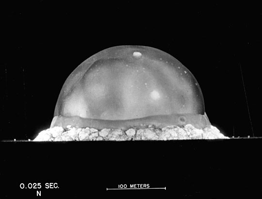
, and from the Life magazine photo he knew the radius of the blast, R, at a particular time, t. That meant he knew everything in this expression except for E, which he was trying to find, and could now solve for E. That’s how Taylor obtained his estimate of 22 kilotons.

I hope this gives you some sense of the power of this approach and also helps you see dimensional analysis as a relatively simple to use tool in the modeler’s toolbox. If you want to explore this further, just let me know. In the meantime, I’ll leave you with a video I often share with my students. I ask them to use this video and dimensional analysis to estimate the gravitational acceleration on the moon.

– John

It’s summer in Delaware and for me that means at least one day spent at Jungle Jim’s, a pretty neat water park in Rehoboth Delaware. While my favorite water ride is by far and away the lazy river, I do enjoy watching this guy:

jungle-jims5


If you haven’t seen one of these before, it’s a “tipping bucket.” Basically, it’s a large bucket on a slightly off center axle with a pipe pouring water into the bucket. The bucket slowly fills, become more and more unstable, and then suddenly dumps all of its water at once on the crowd below. It then returns to its upright position and the process repeats. If you’d like to see one in action, here’s a 30 second video that will give you the idea. Or, you could take a day off and go to the water park. Your choice.

The tipping bucket is really fun to watch. The anticipation builds, you can see the crowd growing more and more anxious, and then “splash!” you get a giant bolus of water and everyone screams in delight. Every time I watch one of these, I’m thinking “periodic function,” “what’s the period?,” “when will the bucket tip?,” “how do the physical parameters of the bucket relate to the period?” and related such questions. These questions, of course, just cry out for a mathematical model!

Now, I’m not going to build a full-blown mathematical model of this system here. I’d encourage you to think about playing with this system yourself and I’m happy to talk further with anyone who’d like to try and develop this as a project for their classroom. Here, I want to point out how this simple water park novelty is a representative of a class of oscillators that are incredibly important in a whole host of areas. I’d also like to talk for a minute about how this fits in with the CCSSM high school standards on functions.

We can pretty easily sketch what a graph capturing the motion of the bucket would look like:

SketchTime_2015_0805_0811_0366

Here, we’ve plotted time on the x-axis and the bucket’s angular displacement from the upright position on the y-axis. For a relatively long time, this displacement changes very little, then, suddenly, there is a rapid change and a rapid reset back to the horizontal position. The whole graph repeats over and over, which we already imagined when we starting thinking “periodic function.” It’s pretty clear however that this isn’t a simple sinusoidal function or any of the other “typical” periodic functions we might talk about in a high school math class. That brings up the question of what the CCSSM intend when they write this:

Interpret functions that arise in applications in terms of the context.

CCSSM HSF.IF.B.4

For a function that models a relationship between two quantities, interpret key features of graphs and tables in terms of the quantities, and sketch graphs showing key features given a verbal description of the relationship. Key features include: intercepts; intervals where the function is increasing, decreasing, positive, or negative; relative maximums and minimums; symmetries; end behavior; and periodicity.*

We didn’t have to look very hard to find an example in an application that doesn’t at all look like the periodic functions they’re studying through the related standards on trigonometric functions. And, here’s where we have an opportunity to really enrich a student’s experience both mathematically and in understanding the applications of mathematics.

If you went no further in class than sketching the behavior of the tipping bucket as we did above and then leading a discussion that drove home the idea that the class of periodic functions is much bigger than the set of trigonometric functions, I’d argue you’ve already done something really important for enhancing their mathematical understanding of functions. You’ve ultimately set them up to better appreciate the magic of Fourier series later on in their studies when they see that all periodic functions can be synthesized from infinite sums of trigonometric functions. (That statement loses some magic for those who think that the only periodic functions are trigonometric functions anyway!)

At the same time, you can also introduce students to the idea of a class of oscillators and help them see the unifying power of mathematics in applications. You’ve likely already showed them multiple systems in the real world that lead to sinusoidal oscillations, now you can introduce the idea of relaxation oscillators and discuss how the tipping bucket is just one particular instance of this class.

Relaxation oscillators are characterized by the behavior we see in the tipping bucket. There is always some slow “build up” phase, a sudden release of energy, and then a return to the start of the build up phase. If you think for a moment, you can probably imagine other instances that you’ve already seen. Here’s another example:

I think it would be fun to challenge your students to go find other instances of systems that demonstrate this slow-build up/rapid release behavior. If you really want to challenge them, you can have them build one of their own:

and, then tackle the modeling problem!

– John

In our professional development, we talk a lot about the notion of “thought tools” and how to wield them. Today, I’d like to talk a little bit about this idea and see if we can clarify the notion of “thought tool.”

We’ve borrowed the language and the idea of “tools for thinking” or “thought tools” from the philosopher and cognitive scientist Daniel Dennett. (In my humble opinion one of the few living philosophers worth listening too. Nick Bostrom is another.) Dennett lays out the notion of though tools in his book “Intuition Pumps and Other Tools for Thinking” and gave a wonderful talk with the same title at Google.

Both Dennett’s book and his talk do a fantastic job explaining this notion in detail, so here, we’ll just introduce the basic idea and then explore what this has to do with the art of mathematical modeling.

Dennett opens his book with a wonderful quote from one of his former students:

“You can’t do much carpentry with your bare hands and you can’t do much thinking with your bare brain.”
– Bo Dahlbom

He then develops the idea of “tools for thinking” by analogy with ordinary tools. Just as we leverage the power of the hammer or the saw or the chisel to expand our ability to do carpentry and expand the range of carpentry problems we can tackle, Dennett argues that we can and should pay attention to the tools we use for thinking about problems. Just like tools for carpentry, thought tools provide us with the opportunity to tackle harder problems and do a better job with them.  So, let’s look at two examples of general thought tools, Sturgeon’s Law and Occam’s Razor.

Sturgeon’s Law is usually expressed as “90% of everything is crap.” That means 90% of papers on molecular biology, 90% of political commentary, and 90% of blog posts on the internet. While the “90” figure isn’t meant to be viewed as a hard and fast quantitative statement, the idea is that in any area, most of what is written or said is, well, crap. The key point is that this statement is also useful for thinking about things. If you’re learning a new subject, don’t waste your time with the 90%, focus on the 10% that’s really good and really important. If you’re a critic, don’t waste our time taking easy shots at the 90%, give us some critical insight into the important 10%. I think this gives you the sense of what a “thought tool” is all about. Generically, it’s a useful way of approaching certain problems.

Occam’s Razor is another such thought tool and likely a familiar one. This one we can state as “Do not multiply entities beyond necessity.” Or, more directly as “Take the simplest theory.” That is, when I flip a switch and a light bulb comes on, I should probably assume an electrical circuit has been closed rather than assume that the switch was a signal for tiny ghosts to light a small fire in the bulb in my lamp. Again, this “thought tool” is a useful way of thinking about and approaching certain problems.

When we think about mathematical modeling, this idea of “thought tools” becomes valuable on two levels. First, the art of mathematical modeling is itself a thought tool. That is, it’s a way of approaching certain types of problems. Just like applying Sturgeon’s Law to the question of what happens when I flip my light switch makes no sense, it’s important to realize and keep in mind that mathematical modeling is a way of approaching certain types of problems. While it’s range of applicability is far greater than that of Sturgeon’s Law or Occam’s Razor, it is still limited, and throwing questions at it for which it’s not equipped is likely to lead to nonsense.

On another level, the idea of thought tools itself gives us a way to think about the teaching and learning of mathematical modeling. Suppose you were observing a philosopher at work and they were asked to choose between the electric circuit or the ghost theory of the light bulb as discussed above. It’s likely they’d, without discussion, simply assume the electric circuit and move on with their lives. It would be up to us to ask “How are you thinking about that?” Such a question would lead us to uncover the idea of Occam’s Razor, which we could then use for ourselves in all sorts of situations. It would then be a heck of a lot easier to teach students about the idea of Occam’s Razor and how to use it than it would be to teach them the answer to every question comparing alternative theories. That is we make more philosophers by teaching students both what to think about and how to do the thinking. But, we as teachers have to carefully observe practitioners and work very hard to understand what is going on with their thinking.

In the same way, we argue that we need to do this with practitioners of the art of mathematical modeling. In a previous post on the modeling cycle, we alluded to this need when we talked about how practitioners don’t really follow a series of steps and how the modeling cycle is only a crude model of the practice. This, in turn, means that there is likely a lot more going on with the mathematical modeler when they are practicing their art. They’re making use of many thought tools that remain hidden unless we work to ferret them out. The modeling cycle gives us some picture, but only in the broadest sense and only of the most obvious of these tools.

As an example, let’s consider “Formulate.” The CCSSM describes this step in their modeling cycle as “formulating a model by creating and selecting geometric, graphical, tabular, algebraic, or statistical representations that describe relationships between the variables.” But, there must be much more to it than that! How exactly do I “select”? Is it like choosing from a menu? Or, is there some other reasoning process involved? How do I “create”? When do I know to “create” versus “select”? Hidden in the practice and in that innocent looking box of “Formulate” there is a heck of a lot more going on.

That’s where this idea of “thought tools” comes back into play. The practicing mathematical modeler has a pretty full toolkit. When they see objects in motion they think “Newton’s Laws” or “F=ma.” When they see a measurable quantity changing with time, they think “conservation law.” And, when they see something in nature choosing a particular shape, they’re likely to be thinking “minimization principle.”

Note that none of these are automatic or inborn and this is where those who would teach mathematical modeling have some work to do. The teacher of mathematical modeling must themselves be a modeler, fill up their toolbox, and be aware enough of what’s in their toolbox that they can identify their thought tools and help equip others in the same way.

As Daniel Dennett says in the opening line to his book – “Thinking is hard.” Similarly, thinking like a mathematical modeler isn’t easy, but thought tools can make the road a little easier to travel.

– John


By now, you’re likely familiar with the modeling cycle introduced in the Common Core State Standards.

160518_3

Today, I want to explore this notion of “modeling cycle” a little bit and urge you to think a little bit differently about this idea. One trend I’ve noticed in the mathematics education community is the deconstruction of this cycle or the listing of the parts like this:

(1) Problem
(2) Formulate
(3) Compute
(4) Interpret
(5) Validate
(6) Report

The point is usually made that these are all related to key skills that the mathematical modeler must possess and I wholeheartedly agree with that idea. It’s when the point becomes “these are all key steps in the modeling process” that I start to grow concerned.

Something I’d urge you to keep in mind as you study the teaching and learning of mathematical modeling is that the modeling cycle is not the same thing as mathematical modeling. Now, that sounds a little funny, so let me say it another way. The modeling cycle is simply a model of the process of mathematical modeling and as with all models, we have to be sure not to confuse the model with thing in and of itself! As with all models, the modeling cycle is incomplete, provisional, rests on assumptions that are open to question, and should be used carefully, with all of these points in mind.

If you’ve ever Googled “mathematical modeling cycle” you’ve likely gotten an inkling of this point and encountered other modeling cycles like this one from the Stepping Stones project at Indiana University:

mathmodcycleOr this one from Rita Borromeo Ferri:

13138_2010_9_Fig1_HTML

Hopefully, seeing these different modeling cycles drives home the point that there is no single “modeling cycle” that is any sense “the” modeling cycle, but rather, they are all just different ways to model the process of mathematical modeling.

Recognizing this distinction, or failing to recognize this distinction, has implications for how we teach the art of mathematical modeling. Don’t fall into the trap of believing that the modeling process can be deconstructed into a list of “steps” to follow! Just as when scientists are doing science, they aren’t holding some poster version of the scientific method in their head and going through a linear process, the mathematical modeler isn’t going through a simple checklist either. More likely, they are moving fluidly between steps in a variety of orders, skipping steps, creating new steps, and doing a whole bunch of things that are represented merely as lines connecting steps in a typical modeling cycle.

The primary implication then for teaching and learning is this – don’t attempt to teach the art of mathematical modeling by having your students mechanically plod through the steps in some modeling cycle! Rather, engage them in mathematical modeling through the joint investigation of genuine modeling situations and later use the modeling cycle as a tool to engage them in meta-thinking about what they did and didn’t do during their investigation. Feel free to use whichever modeling cycle best fits your classroom! And, always keep in mind, that the modeling cycle is after all, just a model.