Some time ago, I had the pleasure of spending part of my summer working with a local high school teacher (Chuck Biehl), an undergraduate mathematics education major (Alexandrea Hammons), and a math education faculty member (Alfinio Flores), on a project we just called the “Bubble Board.” At the time, our interest was in developing a simple hands-on project that Chuck could take back to his classroom and where his students could gather data and learn a few things about curve fitting using a data-set they’d gathered themselves. We wrote this up as an article for the Ohio Journal of School Mathematics. You can find the full article here.
Today, I thought I’d revisit this project and talk a bit about it from the perspective of mathematical modeling. The Bubble Board is a great system in that it’s very simple to build and use, and in that students can gather data using nothing more than a stopwatch, a pencil, and paper. At the same time, the behavior of the system is interesting, and yet mathematically accessible for a wide-range of students.
The Bubble Board was originally designed by the physical chemist, Goran Ramme of Uppsala University in Sweden. Like many scientists before him, from Isaac Newton to Lord Rayleigh, Ramme’s been fascinated with soap films. It was from his wonderful 2006 book, Experiments with soap bubbles and soap films, that I first learned of the Bubble Board.
In designing the Bubble Board, Ramme was interested in devising a way to measure the average lifetime of a soap bubble. You blow a bubble and eventually it pops, but if you blow many bubbles and measure how long it takes each one to pop, what does the distribution of bubble lifetimes look like? Ramme’s Bubble Board gives you a way to blow a whole array of soap bubbles all at once. Here’s a picture of the version of the Bubble Board that we made:
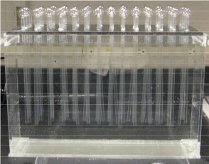
As you can see, the system is simple. You have a latex sheet with an array of 56 identical, evenly spaced holes drilled into the sheet. Through each hole, you place a soda-straw so that about 2cm of the straw pokes through one side and the rest of the straw hangs below. The short end of the straws are then dipped, en masse, into a soap solution creating a flat soap film over the top of each straw. The board is then flipped and the long-end of the straws submerged in a water tank. The water, of course, rises in each straw and the resulting pressure “blows” a bubble at the other end of the straw. You end up with an array of identically-sized soap bubbles.
(Bonus Modeling Problem – How big will each soap bubble be? What is the relationship between how far you submerge the straws in water and the radius of each bubble?)
Now, Ramme approached the Bubble Board from the perspective above. That is, he approached the Bubble Board as a tool for measuring the lifetime of a large array of bubbles simultaneously, thereby building a picture of the distribution of bubble lifetimes and gaining insight into the average lifetime of a soap bubble. We approached the Bubble Board from the point of view of dynamical systems. That is, if you create this array of identical bubbles all at the same time, how does the population of bubbles evolve with time? Or, more simply – How many bubbles will be left at time  ?
?
The dynamical systems perspective brings the Bubble Board into the world of population dynamics. This is of obvious interest in fields like ecology, where one wants to understand how the population of a given species, or group of species, changes with time. The study of population dynamics and the mathematical modeling of these types of problems has led to much beautiful and interesting mathematical work of broad applicability.
So, let’s think about the Bubble Board from this perspective a little bit and think about the Bubble Board from the point of view of mathematical modeling. When we first started building our Bubble Board and still hadn’t conducted any experiments, we reasoned as follows: “Well, if you have more bubbles at any given time, more are going to pop in the next instant of time, so the population of bubbles should decrease in a way that’s proportional to the population at any given time.” In other words, exponentially. That is, we argued that the rate of change of the total bubble population,  , should be proportional to the bubble population:
(1) 
Here, r, is the rate of decay of our bubbles. Well, we’ve seen this equation before in this space and we know that the solution looks like this:
(2) 
Here,  is the number of bubbles at time zero. So, we expected our bubble population to simply exhibit exponential decay. Then, Alex (Alexandria) went to lab and started measuring. Rather than the nice exponential decay we expected, Alex found this:
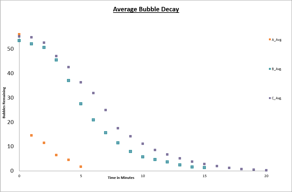
In this figure, the different colors indicate different types of soap solution, but here, let’s just focus on the purple or blue data points. Clearly, the data is not purely exponential. For some reason, the decay curve starts out somewhat flat and then exponential behavior seems to take over and drive the decay. Now, I haven’t put this discussion in the context of the modeling cycle, but hopefully you can see this as an example of how the cyclic nature of mathematical modeling arises naturally through comparison of model prediction and real-world data. We started with our hypothesis about how the system should behave, built our mathematical model and predicted a decay curve that was purely exponential. But, when comparing to the real-world, we see that we were clearly wrong! Well, we got the decay part right and part of the curve looks exponential, but certainly, there is some important behavior in our system that our model is not capturing.
So, we need to go back and revise our model and see if we can glean a deeper understanding of our system. Thinking about our array of bubbles a little more carefully we realize that if it’s true that bubbles have a common average lifetime, then near the start of the experiment very few bubbles should actually be popping. For example, if your average bubble lives for one minute, then near time zero, i.e. the start of the experiment, only a few “outlier” bubbles should pop. Most bubbles should persists and then as time gets close to one minute we should start to see your typical bubble pop. Here, the behavior should look like exponential decay as when your “average” bubble is popping, the number popping should be proportional to the number of bubbles you have. As you get well past one minute, you should again only see your “outlier” bubbles and they too should eventually pop.
How might we modify our mathematical model to capture this behavior? Well, in our original model we assumed a constant rate of decay. We called this constant r and said that for all time our population should decay at this fixed rate. But, now, we’re saying that for short times, this rate should be small and should increase to some constant rate only as time gets close to the average decay time of our bubbles. That is, our look at the data and our new hypothesis about how our population behaves implies a decay rate that varies with time rather than remains constant. Mathematically, we can achieve this by modifying our model like this:
(3) 
If we think about this new term as being lumped together with the rate, r, that is, if we think about this as being our rate:
(4) 
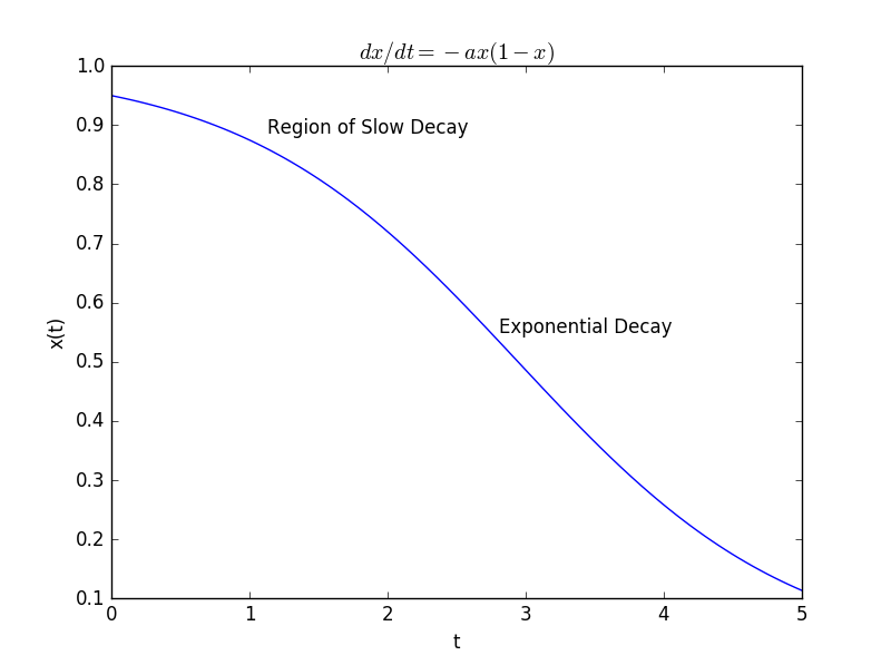
then our rate of decay is small when the population is large, as we expect, and gets larger as the population shrinks. In fact, as the population shrinks, the new term becomes negligible and our model approximately becomes one of exponential decay. This new model is called a logistic model and the solution looks a little different than our previous solution:
(5) 
More importantly, the shape of the decay curve looks a lot more like the one we observed experimentally:
So, we can feel a bit more comfortable in that our model captures the real-world behavior more accurately. Of course, more work remains to be done! How, for example, does the constant  in our new model relate to properties of our soap bubbles? How does the constant
  relate to these properties? Is there some reason to believe our variable rate is the right one?
Hopefully you enjoyed our detour into Ramme’s Bubble Board and can see it as a hands-on way to introduce your students to some interesting mathematical modeling questions and to the broader topic of population dynamics. The system lends itself to investigation by students across a wide-range of mathematical background, so whether you investigate the simple problem of predicting bubble size as a function of the depth the straws are submerged in the water, or the more complex problem of predicting how the population size changes with time, I think you’ll find something here to enjoy.
John

 . Room temperature is
  and initially the potato is at some higher temperature,
  . There are four parameters in the model. The mass of the potato,
  , the specific heat,
  , which measures the amount of energy needed to raise a unit mass of potato one degree in temperature, the surface area of the potato,
  , and the heat transfer coefficient,
  , which measures how fast the potato loses heat energy to the surrounding environment. We note that this model can be thought of as a statement of the principle of conservation of energy. The equation simply says the change in the energy of the potato is equal to the energy lost to the surrounding environment. The left-hand term is this change in energy, and the right-hand term relies upon Newton’s Law of Cooling which says that the energy lost to the surrounding environment is proportional to the difference between the temperature of the body and the temperature of the surrounding environment.

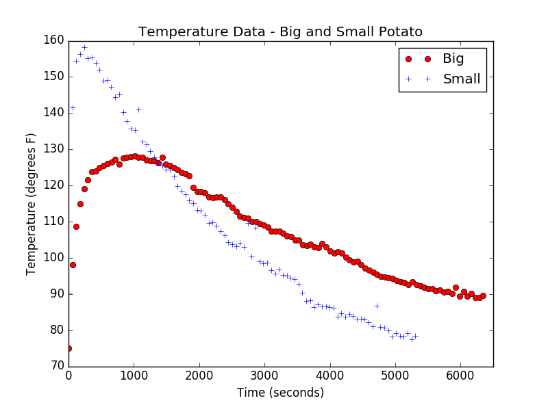
 . For each potato, since they differ in mass and surface area, we’ll have a different
  and for our large potato,
  .If we examine the ratio
  , this ratio will give us our answer. If it’s bigger than one, the small potato must cool faster, if it is less than one, the large potato must cool faster. But, also notice that if we assume our potatoes are made of the same “potato-stuff” then


 ) and a TMP36 temperature sensor (
 ). We wrote Python code to carry out the sensing, gather data every minute, and store the data to a file for later analysis. This let us get lots of data for each potato, carry out the experiment over a long-time (one and a half hours), and not need to be there to monitor the experiment. If you’re interested, I’ve pasted the Python code at the bottom of this post for you to use or copy as you see fit. Now, if you don’t want to go the route of microcontrollers and sensors, all you need to carry this experiment out is a way to measure temperature and a watch. You could use a Vernier temperature probe or even a good old-fashioned glass thermometer. To heat our potatoes we placed each one in the microwave oven for five minutes. We then stuck our probe into the middle of the potato as best we could, sat back, and let our potatoes cool. Here’s our simple setup:
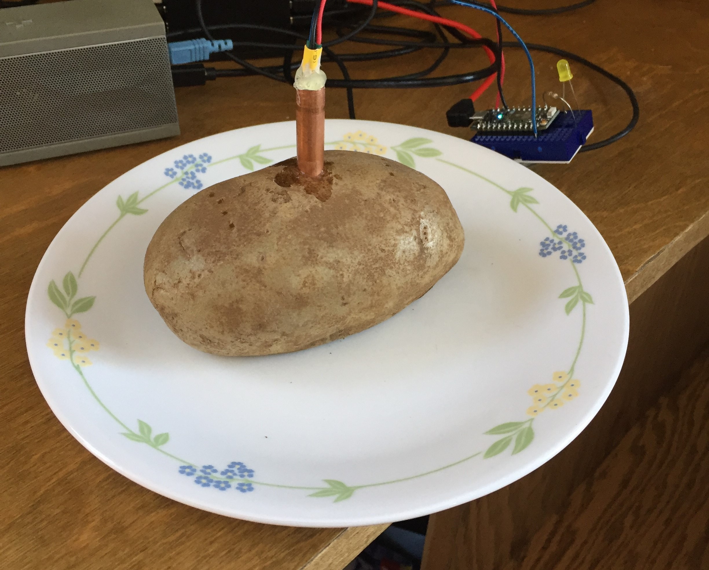
 ?
?