Last week, I had the opportunity to spend a few hours working with folks at Delaware’s Appoquinimink school district. The group was a “STEM Council” composed of district administrators, teachers, principles and others committed to ramping up STEM activity and STEM opportunities in the district. It’s always a lot of fun for me to get to work with such a dedicated group of people and to spend time talking about STEM, modeling, and education. A good portion of our conversation revolved around the intersection of the CCSSM and NGSS and today, I ‘d thought I’d share some of that discussion here.

The NSTA published a Venn diagram that makes exploring the overlap in the CCSS and NGSS practices quite easy:

PracticesVennDiagram_Page_1_000

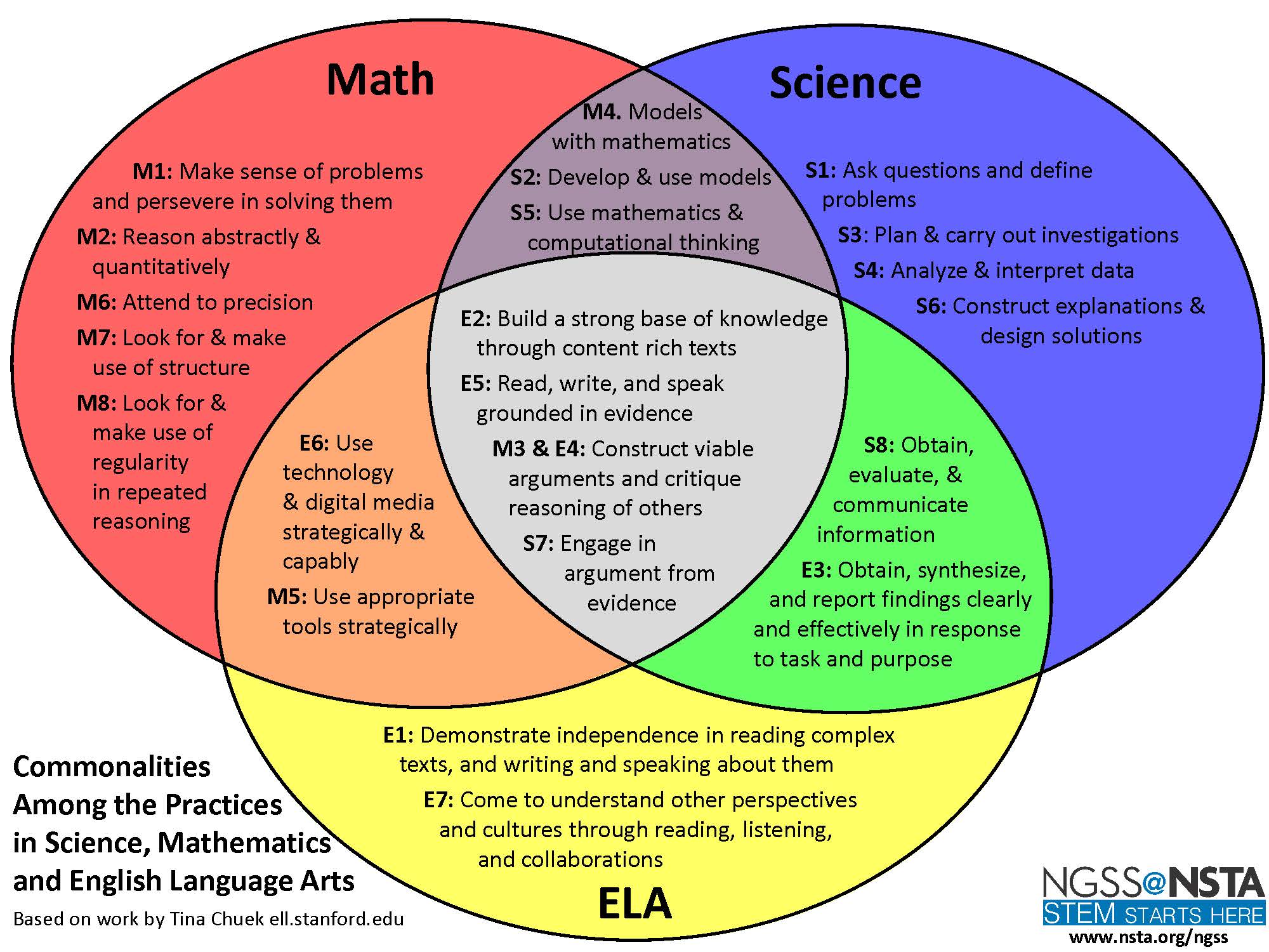
While all of the practices are, of course, crucially important, and while it is interesting to think about all the overlap regions, what’s of most interest to me is the purple region that shows the overlap between the CCSSM and NGSS:

PracticesVennDiagram_Page_1_000

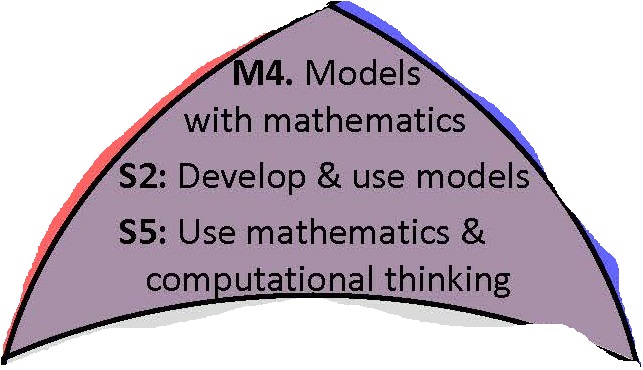
This region is really showing us where the practices of mathematics and the practices of science overlap. It should come as no surprise that this is where the modeling standards live. Readers of this blog are certainly familiar with the CCSSM SMP #4, i.e. “Model with mathematics,” but may perhaps be less familiar with the parallel standard in the NGSS, S2, “Develop and use models.” It’s important to note that S2 is actually broader than SMP 4. When the NGSS says “Develop and use models” they are talking about both mathematical models and other types of models. While one can certainly make a strong argument that mathematical models are the most important types of models that scientists use, it is useful to explore some of these other types of models and to understand a little bit about modeling more generally than as described in the CCSSM.

Why should we bother to think about these “other” types of models? I’ll argue that besides often being useful in and of themselves, having broad knowledge of “models” and “modeling” makes one a better teacher and doer of mathematical modeling. Many of these other models and modeling approaches are more intuitive and more accessible than mathematical modeling and a discussion of these can serve as an entry point into mathematical modeling. At the same time, when we do mathematical modeling, we’re often also, consciously or unconsciously, using other types of models in our process. When I work with groups like Appoquinimink’s STEM Council, we often explore four “other” types of routinely used models so that folks can consciously add these to their toolbox and think about how they use them and how they can be used as part of a mathematical modeling process. Here’s a brief description of the four types of models we talk about:

Scale Models – This is the one with which most people are already familiar and likely the idea that leaps to mind when someone says the word “model.” By scale model, we mean a physical representation of some real world object that is proportionally scaled to some other size. This might be an architect’s scale model of a proposed building, an astronomer’s scale model of the solar system, or a biologist’s scale model of the cell. In each of these cases, the object under study has been represented on a human scale. That is, it’s been built to a size that we can readily deal with visually. It’s been built to a size that we can take in at a glance, see as a whole, and see relevant parts as needed. In building a scale model, one makes decisions similar to those made in any modeling process. We ignore some things and focus on others. We choose what to focus on and what to ignore according as what we’re interested in visualizing or understanding and our models’ utility is dictated by these choices and decisions.

Idealized Models – The notion of an idealized model is certainly one that is used routinely by mathematical modelers, but they also serve as a useful tool for thought experiments in their own right. By an idealized model, we mean one where we conceive of a system as consisting of idealized parts that don’t actually exist in the real world. We might talk about frictionless blocks sliding down frictionless inclined planes or perfectly elastic billiard balls, or perfectly rigid rods, or one-dimensional rods and so on. None of these objects actually exist. There are no perfectly elastic balls or perfectly rigid rods, but if we want to think about the motion of billiard balls or the motion of a pendulum, it is useful to conceive of such idealized objects. We might then draw conclusions just from thinking about systems of such idealized objects (the arc of a perfectly rigid pendulum will lie on a circle) or frequently, the system we conceive of as constructed of such objects becomes the one we mathematize as we build a mathematical model.

Analogical Models – We we think about analogical models, we’re, well, arguing by analogy. We say “A is like B and B behaves as such, so perhaps A behaves in an analogous manner.” If you’re an economist you probably talk about “pumping money into the system” or “turning up the interest rates.” There is no “pump” in the world’s money supply and no knob for adjusting interest rates. What you’re doing is saying the economy is like a machine and money like something that flows through that machine. Pumping and turning knobs then become ways to think about what you are doing to the rather abstract “machine” that is the economy. We’ve talked about “toy models” before and these are too often great examples of analogical models. Our Great Lakes problem had us exploring the flow of a contaminant through three small containers. There, we were arguing that the flow of a contaminant through the Great Lakes behaved analogously.

Phenomenological Models – I always like to draw particular attention to this one because, unfortunately, it is what many people think of as being “mathematical modeling.” And, it’s not identical! Phenomenological modeling is what we do when we fit a curve to data. It’s our way of describing a data set using mathematical objects. We may do this visually or we may use mathematical tools like the method of least squares to do this fitting, but at the end, what we’re doing is describing data. It’s important to realize that we’re modeling data and that this is one step removed from the real world. This is the type of modeling that the CCSSM calls “descriptive modeling,” and so it falls into the class of “mathematical models,” but it’s important to note that it’s but one subclass of mathematical models. An important one, but just a piece of the puzzle.

If you’re a math teacher and you haven’t read the NGSS, I encourage you to do so. At the very least it’s worth reading their description of “Develop and use models.” Working together with our science teacher counterparts is a tremendous way to further the teaching and learning of mathematical modeling and exploring what we have in common (which is a lot!) is a great place to start.

John


In his interesting recent book, Average is Over, economist Tyler Cowan spends considerable time discussing and analyzing the phenomena of “freestyle chess.” While Cowan is interested in the future of the economy, the future of work, and the impact of technology on the workplace, aspects of the freestyle chess movement struck me as a good analog for how mathematical modeling activities should play out in the classroom or in the workplace. So, today, I’d like to explore that notion a bit and introduce the idea of “freestyle math.”

Chess, of course, developed as a competitive game between two players. The relative simplicity of the rules and the absence of chance as an aspect of the game combined with the deep complexity and tremendous variety of possible play has made chess an enduring pastime played by millions for about 1400 years. For most of that time, the standard of play was human vs. human, with exceptionally talented humans becoming “grandmasters,” people who could play at extraordinarily high levels.

In the 1950’s, things began to change. Alan Turing, who we discussed in a previous post on pattern formation, realized that a computer could in principle be programmed to play chess. Turing even developed strategies for such a program and wrote chess-playing code long before the computer hardware side of the world was developed enough to execute such code. However, before long, the hardware side of the world was up to speed and by the 1970’s one could purchase a dedicated chess-playing computer that looked like this:

chesschamp4

I recall an uncle of mine owning one of these early machines and I recall being amazed that the computer could pretty handily beat everyone I knew. But, at that time, at least, really good humans were still far better than the best chess playing machines. This too changed rapidly and in 1997, a computer called Deep Blue, developed by IBM, beat the reigning world chess champion, Gary Kasparov, 3 1/2 to 2 1/2 in a six game match. (Note that 1/2 points are awarded to each side in a draw.)

In the last eighteen years, computers have only gotten better at chess and humans, well, haven’t. Today’s most talented players don’t stand a chance against a good chess program and a good chess program can now be a single app on the phone in your pocket. However, shortly after losing to Deep Blue, Kasparov asked an interesting question – What would happen if instead of human vs. human or man vs. machine the competition were man + machine vs. man + machine. The new competitive sport of “freestyle chess” was born soon thereafter.

In this incarnation, chess is a team sport, where members of the team may be computer programs. In fact, in freestyle chess pretty much anything goes with Kasparov having remarked “Even if they were assisted by the devil, that would probably be covered by the rules.” And, in freestyle chess, something remarkable happened. Human-machine teams could defeat a single top-ranked chess playing computer program. The level of chess played by these man/machine hybrid teams was now higher than that played by either man or machine alone in the past.

Cowan describes freestyle chess matches as a being like a beehive of frenetic activity with human teams scurrying from computer to computer, combining, and analyzing suggested moves from multiple analyses before making a final decision. He also notes, interestingly, that the best freestyle teams are not necessarily made up of top chess players working with top chess computer programs. Rather, a strong freestyle team needs humans with a very different skill set. Yes, they have to understand chess and the basic elements of play, but they also need to understand computer programs, how they work, what their limitations are, what their strengths are, and how to combine the brute-force “number crunching” approach of computers effectively with human intuition.

As I read Cowan’s description of freestyle chess, I was struck by how similar the activity he described is to the activity of an effective student team working on a mathematical modeling investigation. So, I’d like to encourage you to think of mathematical modeling in your classroom as “freestyle math” and I’d like to explore for a moment some of the characteristics of what that might look like. I’m encouraging you to think of “freestyle math” in this “anything goes” sort of mindset. That is, students should be free to tap into the internet, simulation, textbooks, friends, etc., without bound. The focus should be on the goal of understanding the phenomenon they are investigating and in how one gets there, anything should be fair game. So, here are five characteristics of freestyle chess that I believe map in a one-to-one fashion to freestyle mathematical modeling:

The humans know something, but might not be super-experts

In freestyle chess, the human members of the team are not necessarily grandmaster level chess players or even master level chess players. But, at the same time, they know the rules of the game, have an understanding of strategy, and generally play as well as a decent club player (someone who plays regularly). On a modeling group in the high school classroom you want your “players” to have a roughly similar level of expertise in mathematics and have some expertise in the application area they are investigating. You don’t need a team full of math-whizzes, but you do need your students to take ownership of the mathematics, have a comfort with using mathematics, and be able to know what they need to learn.

Collaboration is key

As in freestyle chess, in freestyle math, the ability to collaborate effectively, both with other humans and with computers is a key skill. The ability to work with a diverse team is important and students also need to know how and when to use technology in their investigations. This means our students need to know when to “Google” and when to think. They need to know when to analyze with pencil and paper and when to turn to the computer.

The humans understand the strengths and limitations of computers

An essential skill of freestyle chess players is knowing both the strengths of various computer programs and the limitations of various computer programs. This is at least as important of a skill for mathematical modelers to possess. They should know to turn to the computer to fit a curve to a data set consisting of even a mildly large number of data points. At the same time, they should know what the computer is doing when it is fitting that curve, what assumptions they are making when they take that curve as being predictive, and exactly where the limitations are in what the computer is telling them. I can’t emphasize this one enough – to use a tool effectively you have to know both what it is good for and what it isn’t.

The humans are able to tap into and filter vast quantities of information

In freestyle chess, humans also bring the ability to both gather vast quantities of information and to filter this information. Freestyle math needs the same skill. Even a discerning Google search about a real-world scenario that students might investigate will return hundreds of thousands of links. Students need to be able to quickly and efficiently zoom in on the relevant information and know what information to trust and what to ignore. At the same time, a simple computer simulation can also quickly return reams of data. Students need to know how to organize this information, how to visualize this information, and again pick out what is relevant and what isn’t.

The humans supply creativity and intuition

Humans clearly bring both creativity and intuition to the table and both of these skills are required in abundance in freestyle chess and in freestyle math. In mathematical modeling, decisions, false starts, retrenchments, intuition, and creativity are the norm. Students need to be able to offload to a computer the things it does best and bring to the table the sorts of creative approaches and intuition that they do best.

As you work to engage your students in the practice of mathematical modeling I’d encourage you to think “freestyle math” and look to freestyle chess as a model for what open collaboration between people and between man and machine can produce. I’d also encourage you to think about the skills that such activities demand that go beyond the simple mastery of mathematical procedures, and how freestyle math demands a deep understanding of concepts and the ability to integrate that knowledge in the pursuit of understanding the world.

John


Often in mathematics, and certainly often in mathematics class, we think in terms of direct problems.  That is, we’re given something to “solve,” we’re required to find a path to a “solution,” and that’s where we end up. For example, we might be asked to find the solutions of the following equation

x^2 + 2x + 1 = 0

and we proceed by using the quadratic equation or completing the square or some such method, and arrive at values for x. If we think of this in terms of applications, we often pose direct problems as well. Here, for example, we might say, suppose we drop a ball from a height h, we assume air resistance is negligible, how fast is the ball traveling when the ball hits the ground? Or perhaps, how long will it take the ball to hit the ground?

But, often, in the real world, our problems aren’t formulated like this. Rather, we’re faced with problems that are posed the other way around. That is we’re faced with what are called inverse problems.  In these problems, what we’re given is the solution and what we have to do is figure out where it came from. You’re likely familiar with such problems, but perhaps haven’t thought of them in this way before. One common example is the “sonar problem” or the problem of echolocation. If I’m a bat, what I do is make a noise, and then listen for the reflected sounds that come back to me. What I then try and do is figure out the direction, location, and perhaps shape, of the objects in the environment that caused the particular patterns of reflected sounds that I heard. That is, I’m given the solution, i.e. the reflected sounds I measured, and have to figure out the problem, i.e. what pattern and shape of objects in the environment would cause that set of reflected sounds?

Such problems are an important class of problems that the mathematical modeler must be equipped to deal with. And, such problems, can be a source of challenging and engaging problems for students learning the art of mathematical modeling. Today, I’d like to explore a few simple versions of such problems and how you might use them in your classroom.

One of my favorites is a problem that was posed by Isaac Newton in Universal Arithmetik and was discussed by Groetsch in his text Inverse Problems: Activities for Undergraduates. Newton posed the problem like this:

A Stone falling down into a Well, from the Sound of the Stone striking the bottom, to Determine the Depth of the Well.

The unusual capitalization is Newton’s and apparently the style of the time was to state commands rather than pose questions. Today, we might state the problem as:

Can we determine the depth of a well by dropping a stone into the well and listening for the sound of the stone striking the bottom?

Why is this an inverse problem? Well, what we’re asked to do here is to take information we obtain at the end of a process, i.e. the time interval between us releasing the stone and it us hearing the stone strike the bottom of the well, and to infer how the stone must have traveled and from this deduce the depth of the well.

This particular inverse problem can be approached by solving the direct problem, which requires us to build a mathematical model of the time which elapses between the release of the stone and us hearing the sound of the stone striking the bottom of the well. We can imagine that we release the stone and start a stopwatch at the same instant. When we hear the sound, we stop our stopwatch and call that elapsed time, t_m. Further, we can suppose that t_m can be divided into two parts, the time it takes the stone to fall, t_f, and the time it takes the sound to travel back up the well, t_s. Our measured time is then the sum of these two:

t_m = t_f + t_s

Our job is then to build a model of the fall and the travel of the sound that lets us express t_f and t_s in terms of the depth of the well, h. It’s worth noting that both modeling the fall and understanding the fact that sound travels at a finite speed fall within the scope of the NGSS standards and so, should be within reach of the high school classroom. I’ll skip the details here, but you should be able to arrive at an expression that looks like:

t_m = (2h/g)^{1/2} + h/c

Here, g is the gravitational acceleration and c is the speed of sound in air. A quick plot of t_m as a function of h yields: (plot prepared with Desmos)

g7gmgpouwv (1)

Now, given a measured time, t_m, all one needs to do is draw a horizontal line on this plot at that value of time, find the intersection point with the curve shown, and read off the value of h, the predicted depth of the well. It’s  worth a conversation as to whether or not the h/c 
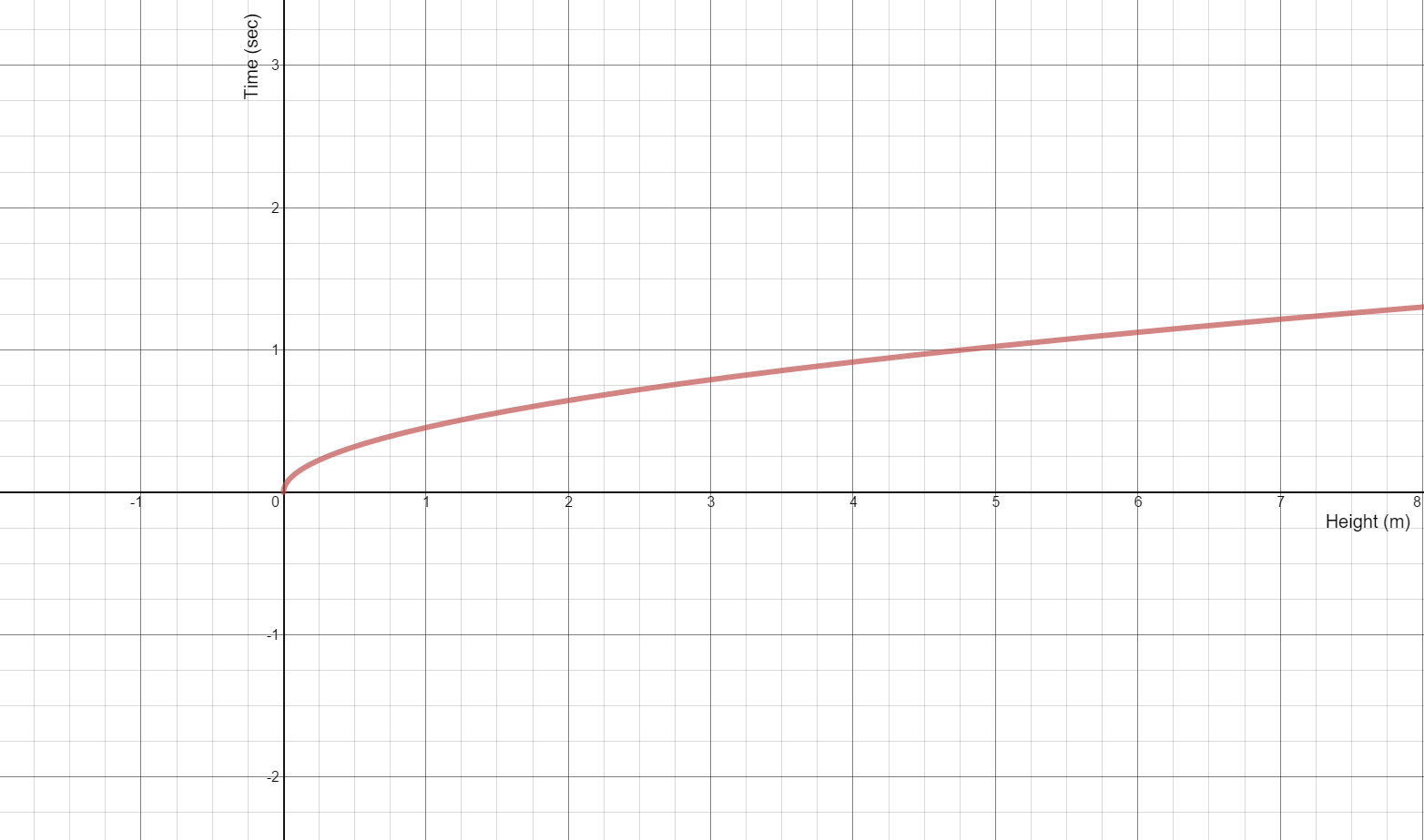
term is important here or when it may be important. It’s also worth taking time exploring how an error in the measurement of t_m translates into an error in the prediction of h. The sensitivity to such error that one sees in this problem is a typical feature of inverse problems.

If you do decide to introduce your students to the notion of inverse problems, it is worth spending at least a few minutes sharing with them the many areas of application where such problems arise. I’d suggest focusing on medical imaging as this is likely familiar territory in some sense, but unfamiliar territory in the sense of them understanding that most of modern medical imaging rests on building mathematical models and solving inverse problems.

I’ll leave you with one last inverse problem that is readily understood, but challenging to investigate. Imagine I tell you that I have a container of some sort but that I’m going to keep that container hidden in a box and not let you see it directly. However, what I will do is pour any volume of water you’d like into the container and tell you the height to which the water fills this hidden container for that volume. I’ll do this as many times as you’d like and give you as much data of this form as you want. The question is then this – can you tell me the shape of my container? Suppose I told you the container had rotational symmetry. Would that help?

I hope that this small taste of inverse problems has inspired you to consider this very important class of problems as you work to build mathematical modeling into your classroom practice. As always, we’d love to hear about your successes and challenges with this or other mathematical modeling investigations.

John