Well, the last few months of 2016 went by much too quickly and unfortunately left me with little time to post. But, it’s a New Year, and I’m anxious to get back to talking about mathematical modeling. So, Happy New Year! Now, let’s get back to work.
Recently, I found myself thinking about several points that we’ve explored in earlier posts. One of these, explored in “Caught or Taught?“, is the idea that mathematical modelers often draw upon a library of canonical mathematical models that they have at their fingertips when they approach a new problem. That is, they often reason by analogy, and use situations and models with which they are familiar as a starting point for thinking about new, unfamiliar, situations. The second point that’s been on my mind is the one explored in “Arduino as a simple tool for hands-on modeling activities,” and is the idea that the widespread availability of low-cost microcontrollers and sensors opens up new possibilities for hands-on activities in the modeling classroom. For many years at the University of Delaware, I’ve taught a mathematical modeling course where we’ve had students engage in hands-on experiments in our own laboratory. I’m constantly amazed that experiments which cost us thousands of dollars to perform just ten years ago can now be carried out at home on your desktop with just a few dollars in equipment.
So, today, I thought I’d explore a canonical mathematical model, but do it in a way that was hands-on and made use of accessible, low-cost technology. Along the way, I’ll point out some problems where you and your students can explore further. The basic mathematical model, exponential decay, is one with which you’re surely familiar, and is in-fact, one of the “starred” domains in the Common Core State Standards. Of particular relevance are the standards:
Distinguish between situations that can be modeled with linear functions and with exponential functions.
Recognize situations in which a quantity grows or decays by a constant percent rate per unit interval relative to another.
Interpret the parameters in a linear or exponential function in terms of a context.
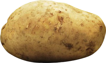
To carry out this project, I enlisted the aid of my daughter, Julia, and this weekend, we spent time playing with potatoes. What more could a high-school student ask from their weekend? The question that we sought to answer was this – Which cools faster, a large potato or a small potato? Somewhat surprisingly, when we polled a few unwitting participants as to their answer to this question, two schools of thought emerged. One school of thought held that the small potato would cool faster as it “held less heat” and hence as it shed energy its temperature would drop faster. The other school of thought held that the large potato would cool faster as it had a larger surface area and that the rate of its losing energy would be hence be greater. Who’s right?
To explore this question, we decided we’d first build a mathematical model and try and make a prediction. Then, we’d design and carry out an experiment, compare, and see if we could both demonstrate an answer and understand why potatoes behave however they behave. For our model we were, of course, treading well-trodden ground. Examine the index of any introductory calculus textbook or any introductory physics textbook and you’ll find an entry for “Newton’s Law of Cooling.” Turn to the page referenced and in the calculus text, you’ll find yourself in the chapter or section on exponential and logarithmic functions. This goes back to our earlier point about canonical models. This mathematical model is certainly not new, but the idea that systems exhibit exponential growth or decay is so useful and encountered so frequently, that it is worth exploring models like these, deeply. So, without extensive derivation, here’s our mathematical model for the temperature of a potato:
(1) 
Here, the unknown is the potato temperature,  . Room temperature is
  and initially the potato is at some higher temperature,
  . There are four parameters in the model. The mass of the potato,
  , the specific heat,
  , which measures the amount of energy needed to raise a unit mass of potato one degree in temperature, the surface area of the potato,
  , and the heat transfer coefficient,
  , which measures how fast the potato loses heat energy to the surrounding environment. We note that this model can be thought of as a statement of the principle of conservation of energy. The equation simply says the change in the energy of the potato is equal to the energy lost to the surrounding environment. The left-hand term is this change in energy, and the right-hand term relies upon Newton’s Law of Cooling which says that the energy lost to the surrounding environment is proportional to the difference between the temperature of the body and the temperature of the surrounding environment.
Now, we know that the exponential function is this very special function whose rate of change is everywhere proportional to itself. Our mathematical model says that the function we’re after, , has this property that its rate of change is everywhere proportional to itself. Hence, our mathematical model is easily solved for :
(2) 
We see that the rate at which our potato cools is exponential, yes, but more importantly, how fast this decay happens for a particular potato is governed by the ratio of the four parameters in our problem:
(3) 
Recall that we want to know whether a “big” potato will cool faster or slower than a “small” potato. The answer lies in interpreting our model and in particular, in interpreting  . For each potato, since they differ in mass and surface area, we’ll have a different . Suppose we call the for our small potato
  and for our large potato,
  .If we examine the ratio
  , this ratio will give us our answer. If it’s bigger than one, the small potato must cool faster, if it is less than one, the large potato must cool faster. But, also notice that if we assume our potatoes are made of the same “potato-stuff” then and are the same for each potato, so this ratio only depends on a combination of potato masses and surface areas. In particular, this ratio reduces to:
(4) 
Here, the subscripts denote the small and large potatoes, as above. So, off to the supermarket we traveled where we bought two standard baking potatoes, one large, one small. The masses were easy to measure with our kitchen scale:
(5) 
But, how to measure potato surface area? (Here’s a problem for further exploration. How do you compute the surface area of a potato? How do you measure it?) I left Julia to tackle this question and she decided that this:
rather resembled this:
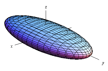
and after some measurements and computations arrived at:
(6) 
Putting this all together, we arrived at:
(7) 
and hence our mathematical model leads us to predict that this particular small potato should indeed cool faster than this particular large potato.
Our next step was to conduct some potato experiments. But, before we go there, let me point out another problem for future exploration. We’re making a prediction for our particular two potatoes. In this case, we predict that the small potato should cool faster than the large potato. But, is this always going to be the case? Surely, if we took our large potato and stretched it out into something resembling a giant French fry it would cool faster. Wouldn’t it? How does our ratio, , depend on potato shape? Can you find two potatoes that you would call “large” and “small,” where the large potato should cool faster?
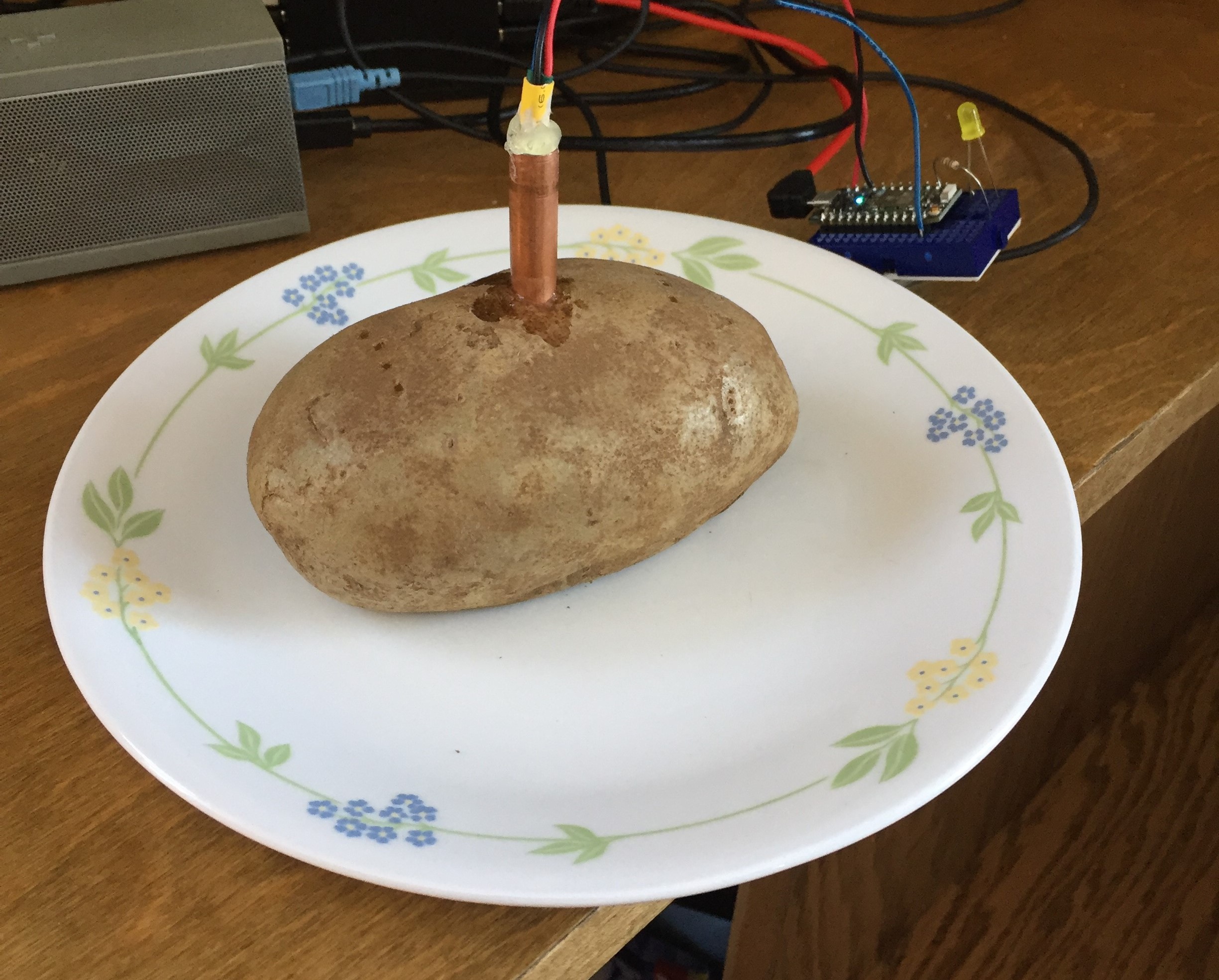
Now, on to experimental potatoes. For our experiment, we used a low-cost microcontroller called a Particle Photon ( ) and a TMP36 temperature sensor (
 ). We wrote Python code to carry out the sensing, gather data every minute, and store the data to a file for later analysis. This let us get lots of data for each potato, carry out the experiment over a long-time (one and a half hours), and not need to be there to monitor the experiment. If you’re interested, I’ve pasted the Python code at the bottom of this post for you to use or copy as you see fit. Now, if you don’t want to go the route of microcontrollers and sensors, all you need to carry this experiment out is a way to measure temperature and a watch. You could use a Vernier temperature probe or even a good old-fashioned glass thermometer. To heat our potatoes we placed each one in the microwave oven for five minutes. We then stuck our probe into the middle of the potato as best we could, sat back, and let our potatoes cool. Here’s our simple setup:
And, here’s our data:
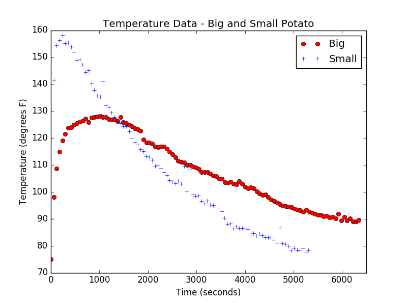
As you can see, the small potato achieved a higher temperature initially, but, as predicted, cools at a faster rate. Since we placed each potato in the microwave for the same length of time and the small potato has smaller mass, it makes sense that its initial temperature should be higher. The transient behavior at the start also makes sense – it takes time for the probe to get to potato temperature. It’s exciting to see that our model and our analysis of yield a correct prediction about which should cool faster. By this point, Julia’s potato-patience was wearing thin, so we left further analysis for another day. But, here’s one final suggestion for exploration for you and your students. If you take the data above (or your own data) and fit an exponential to the exponential part of the curve, your fit will give you an experimental value of for that potato. If you take the ratio of the two values, how close do you get to  ?
?
Well, I hope you’ve enjoyed thinking about this canonical mathematical model and thinking a bit about hot potatoes. Best wishes for a fun year of mathematical modeling!
John
[code language="python"]
#Code for temperature monitoring using Particle Photon
#Using TMP36 temperature sensor with Photon
#Using standard wiring, red -> +3.3V, black -> GND, blue -> A0
#Reading is taken from A0 and converted to a temperature reading
#Note we had to install package spyrk via pip install spyrk

#Here is how to access the Particle Cloud

#Should be able to call via the access token for the system
ACCESS_TOKEN = 'YOURTOKENHERE'
#Or can use username and password
USERNAME = 'YOURUSERNAME'
PASSWORD = 'YOURPASSWORD'

#To create a connection to Python Code
from spyrk import SparkCloud
spark = SparkCloud(USERNAME,PASSWORD)

#Other packages we will need
import sys #Used to break the script if device not connected
import time #Used for delays and to assign time codes to data readings
import numpy as np #Used for creating vectors, etc.
import statistics as stat #Used for computing median, etc.
import matplotlib.pyplot as plt #For plotting
import csv #For writing data to a csv file

#First we will test the connection to the device and terminate the script if not connected
#If connected we alert the user and continue
if spark.YOURDEVICENAME.connected != True:
 sys.exit("Device Not Connected")
elif spark.YOURDEVICENAME.connected == True:
 print("Device Connected")

#Now we will open a file for the temperature data
with open('temp_data.csv', 'w', newline='', encoding='utf8') as csvfile:
 filewriter = csv.writer(csvfile, delimiter=',', quotechar = '|', quoting=csv.QUOTE_MINIMAL)
 filewriter.writerow(['Time','Temperature'])

#Now we construct a function that will read A0 and return temperature
#Note the user calls this function by passing read_length which is the number
#of samples the function will take. The temperature computed from the median of these samples is returned to
#the user. That is, this function applies basic median filtering to the measurement.
def read_temperature_F(read_length):
 work_space = np.zeros(read_length) #Creates an empty vector of length read_length
 for i in range(0,read_length): #This for loop reads read_length number of samples and puts them in work_space
   A0=spark.YOURDEVICENAME.analogread('A0')
   temperature = (9/5)*((A0*3.3)/4095 - 0.5)*100 + 32
   work_space[i] = temperature
 temperature = stat.median(work_space) #Finds median of readings and returns median value
 return temperature


#Now we want to set up a basic data gathering and plotting system for temperature readings
#We'll decide how many samples we want to take and how long between samples. Then, we'll gather
#those samples with time data as well and plot the temperature versus time
samples = 30 #We're going to take this many data points
time_delay = 55 #We'll allow time_delay seconds to elapse between measurements
temperature_data = np.zeros(samples) #Creates a vector for our temperature data
time_data = np.zeros(samples) #Creates a vector of same length for time

#This loop does the measurements
for i in range(0,samples):
 temperature_data[i] = read_temperature_F(8)
 time_data[i] = time.clock()
 print("Sampled temperature is", temperature_data[i], "at time", time_data[i])
 with open('temp_data.csv', 'a', newline='', encoding='utf8') as csvfile:
   filewriter = csv.writer(csvfile, delimiter=',', quotechar = '|', quoting=csv.QUOTE_MINIMAL)
   filewriter.writerow([time_data[i],temperature_data[i]])
 time.sleep(time_delay)

#Now, we plot the results
plt.plot(time_data,temperature_data,'ro')
plt.axis([0,time_data[samples-1],60,80])
plt.xlabel("Time (seconds)")
plt.ylabel("Temperature (degrees F)")
plt.title("Temperature Data - Particle Photon and TMP36 Probe")
plt.show()
[/code]
So this is what I was reading over your shoulder! As always, insightful and humorous. But you did get one thing wrong: I always have patience for potatoes (cooked or not). Looking forward to reading some more posts!
John
Great example for modeling. I wonder if part of the simplification in modeling lies in the assumption of treating the potato as a homogenous mass rather than heterogeneous mix of potato mass and water, both of which heat and cool at two different rates. I also wonder if the overall shape of both potatoes have to have similar shape since the heat dissipation is along the radial direction from the center and if one is elliptical and other spherical i.e. some ratio of the radii needs to taken into consideration. Now of course, one makes it a more complicated model and defeats the purpose of the lesson you were trying to convey.
Bottom line – I enjoyed reading it :- ). Excellent website.