Perhaps the one question we’re asked most frequently by teachers preparing to integrate mathematical modeling into their classroom is “Is this mathematical modeling?” Usually, the teacher has a specific activity in mind and what they really want to know is “Will doing this activity require my students to engage in the full process of mathematical modeling?” Before I go any further, let me say – not every task that supports the development of modeling skills, needs to engage students in the full process of modeling. We’ll explore that in another post, but just keep in mind that here, I’m talking only about those tasks that are designed to have students engage in the full process.
Unfortunately, I don’t think there is an easy or simple to use “litmus test” to answer the question “Is this modeling?” I do think however, that we can list several tests that together tend to catch most of the key points of confusion. So, here are four things you should think about or ask yourself if you’re wondering if the task in front of you is a mathematical modeling task.
Can you find the “why” or the “how” question?
While mathematical modeling “tasks” are generally not cleanly formulated as one-line questions, if you think about your task, you should be able to see your way through to at least one central question you are aiming at answering. Try to find this central question and then ask yourself if your central question is a “why” or a “how” question. If it is, this is a good sign that your task is mathematical modeling task. If you can envision how a mathematical model will help you answer that question, even better! Let’s think through an example to try and clarify this point. A few days ago we discussed the “Great Lakes Problem.” Recall, that the idea was to investigate pollution in the Great Lakes (or your favorite local body of water). That starts out so “open” that there isn’t even a question there at all! But, we “banged that down” to a toy model where we were asking “If we stopped all pollution into lake X, how long would it take for pollution levels to reduce to some level?” That’s a “how” question and a good indicator that you’ve potentially found a mathematical modeling task. Or, consider the discussion around the “tipping buckets” system. There, we were asking “Why is the period of oscillations X and not Y?” Again, a good indicator of a modeling problem.
Will your model have explanatory or predictive power?
Remember, we build mathematical models for a reason. That reason is generically to be able to explain something we see or to be able to predict (and perhaps control) what will happen next with a given system. If you try and envision the model coming out of your task, ask yourself whether it will have this predictive or explanatory value. Again using the Great Lakes problem as an example, the model there would let us predict how long it would take pollution levels to reach some value under certain conditions. That’s a clear testable prediction. In the tipping buckets problem, a good model would help us explain why the period of oscillation is as observed. It would also let us predict what the period would be if we changed the inflow rate of water or other parameters in the system. If the models you envision don’t have predictive or explanatory power, it’s probably not a modeling problem. Now, note, this does depend on the type of model you are imagining your students will construct. If you are envisioning a purely descriptive model, you of course will not see explanatory value. But, you should see predictive value, albeit limited by the nature of descriptive modeling.
Do you already have in mind one right answer?
If you do, this is probably a sign that this isn’t a mathematical modeling activity. Remember that when constructing a mathematical model, the modeler is making assumptions and decisions along the way. These choices lead down different paths and consequentially result in models that look different from one another. You should be able to imagine students constructing different models while engaged in your activity. You should also be able to imagine that some of these models are better than others and have an idea in mind as to what makes a better model for your situation. Is it more successful in terms of making predictions? Does it explain more of what is observed? If you can only imagine one path to one answer that you have in mind, it’s probably not a modeling problem.
Is it clear what validating your model against the real world would mean or look like?
The ultimate test of any model is whether or not it accurately captures that aspect of the real world it was intended to capture. To test that, at some point, the modeler has to validate their model against real world data. Does the model predict accurately what actually happens in the real world? Is it able to explain and account for the full range of observations about the real world system? When you are thinking through your task, ask yourself “If a student created a model of this situation, how would we know if it is any good?” If there is no way to objectivelycompare the model to the real world, this is probably not a modeling problem.
Hopefully, asking yourself these four questions will help you determine whether or not you’re on the right track with your modeling tasks. Please feel free to send along any questions you might have or tasks you would like input on. We’re happy to help!
Last week, I had the pleasure of listening to an interesting talk by Michael Lach of the Center for Elementary Mathematics and Science Education at the University of Chicago. Michael did a very nice job of describing the national picture in mathematics and science education and in relating that picture to efforts localized in Delaware. But, one strong point that Michael made stuck with me above all the rest. He simply said “This is different.”
Michael, of course, was referring to the CCSSM. If you’ve read the standards, you know that they make the point about being different quite forcefully.
These Standards are not intended to be new names for old ways of doing business. They are a call to take the next step.
I’ve read that before, quoted that before, and thought about that before, but this time, I was inspired to think about it while in the middle of conducting professional development on mathematical modeling. Of course, the practice standard “Model with Mathematics” is itself different from past standards documents. But this time I got to wondering about the finer grained implications of that. What is so different about teaching mathematical modeling compared to teaching purely mathematical content?
Well, the answer is that there are a lot of differences. Today, I want to talk about two of these differences that I hadn’t thought about before. Unlike other lists of differences I’ve made that could just as easily be seen as lists of challenges, both of these differences, I believe, are incredibly positive and hopefully exciting for all the new modeling teachers out there.
The first I’ll call “No floor, no ceiling.” Often, you hear those in the math education world talking about tasks that are “Low floor, high ceiling.” I’d like to argue that mathematical modeling projects are even more wide-open than “low floor, high ceiling” tasks and that this should be exciting both for teachers and for students. Of course, it could be terrifying! It could induce in you the kind of vertigo I feel when I see this picture:
But, hopefully you’ll find it more invigorating than terrifying. So, why do I argue that mathematical modeling activities are inherently “No floor, no ceiling”? Let’s think about the floor first. Any genuine mathematical modeling activity starts in the real world. It starts with observation of some pattern or phenomenon. While teasing out a viable modeling problem from this observation takes some skill and guidance, the observation itself makes the starting point wide-open to anyone. Pollution in a lake, tipping buckets of water, the spread of a disease through a population, or the motion of a projectile are all things to which students can easily relate. They have different levels of familiarity with any of these, but a simple picture or video gives them all an immediate way into the discussion. This is part of what the fact that modeling activities are “open” implies. They’re open in the sense of not being well-defined, yes, but they are also open in the sense of at least the start of the discussion being readily accessible to anybody. Modeling activities help us introduce students to phenomena in the real world that are objects worthy of scientific investigation. At the same time, I’d argue that in addition to being open good, modeling activities are also inviting. Not only are they “no floor,” but there is also a big neon sign saying “Come on in!” right at the front. And, once you’re in, there is virtually an unlimited number of ways to proceed, things to investigate, and avenues to explore.
At the same time, modeling activities are also inherently “no ceiling.” A model is always provisional and can always be improved. This is just plain built in to the iterative nature of the modeling process and in fact, into the nature of scientific investigation. No scientist views their mathematical model as being “done.” They might view it as “good enough for now” or “I’ve taken it as far as I can go,” but there is always that very real sense that there is more to be learned, more to be investigated, and more to be understood. Okay, the “high ceiling” in “low floor, high ceiling” is usually interpreted as meaning that you’re only limited by the extent of your own mathematical knowledge or abilities. That, of course, is similar in mathematical modeling. But, the reason I’d still argue that modeling activities are “no ceiling” is because you can always learn more about the real world situation, enriching your understanding, and then come back and use your mathematical knowledge (however limited) in new ways. At the same time, as you learn more math, you can also often come back and investigate the real world in new ways. There might be some sort of a ceiling, but but you can certainly keep climbing up in different points in the room.
The second difference that I want to talk about is around assessment. Assessing mathematical modeling activities is different, not straightforward, and we need to do a lot more work to figure out how to do this well. Yet, at the same time, some of these differences are actually opportunities to create a different environment in our classroom. One of the perennial struggles of the math teacher at any level is designing new quizzes and new exams. How many hours have we spent collectively designing new exams solely because we are afraid that last year’s exams might be “out there”? Mathematical modeling creates an opportunity to treat “last year’s work” in a fundamentally different way. Rather than something to be hidden, the work of previous students on a modeling problem can be viewed as something to be shared. When I teach mathematical modeling courses and decide to have students tackle a problem I’ve used before, I give them the final reports prepared by previous students. I treat these as part of the scientific record, just as I would any journal article. This gives me the opportunity to help students read something very relevant with a critical eye. It helps me show them how science builds on past science. It helps me explain that not everything that’s written is right. So, I would argue that even though assessment of mathematical modeling feels like a challenge, there are very real ways to view it as an opportunity.
I imagine that if you are preparing to incorporate mathematical modeling into your classroom, you’re feeling some trepidation. I hope you can take away from this note some really good reasons to approach this with excitement as well.
In the CCSSM several of the “starred” high school standards relate to quantitative reasoning and using units to solve problems:
Reason quantitatively and use units to solve problems.
CCSS.MATH.CONTENT.HSN.Q.A.1
Use units as a way to understand problems and to guide the solution of multi-step problems; choose and interpret units consistently in formulas; choose and interpret the scale and the origin in graphs and data displays.
CCSS.MATH.CONTENT.HSN.Q.A.3
Choose a level of accuracy appropriate to limitations on measurement when reporting quantities.
Modeling Standards: Modeling is best interpreted not as a collection of isolated topics but rather in relation to other standards. Making mathematical models is a Standard for Mathematical Practice, and specific modeling standards appears throughout the high school standards indicated by a star symbol (*).
By the presence of the star, as the footnote in the CCSSM indicates, we know that this particular set of standards is of special importance to the practice standard, “Model with mathematics.” In any modeling process, paying attention to units, constantly checking that model equations are consistent in terms of units, and defining appropriate quantities are all crucial skills. Today, I’d like to explore the related skill of “dimensional analysis.” This is a skill that is pretty typically in the toolbox of the practicing mathematical modeler, yet, hasn’t seemed to make its way to the high school classroom.
It’s easiest to illustrate the idea of “dimensional analysis” with a story and as with many stories around mathematical modeling, this one revolves around the great G.I. Taylor. Taylor was an incredibly prolific physicist and mathematician (1865-1975) the bulk of whose work was in fluid dynamics, but who possessed a wide-ranging mind, and made fundamental contributions to multiple areas of study. The “FRS” at the end of his name and the “Sir” at the beginning might give you some idea of the impact of his work. His biographer, George Batchelor, himself a very notable scientist, described Taylor as “one of the most notable scientists of this (the 20th) century.”
This particular story about Taylor takes place in 1950, shortly after the development of the first atomic bomb. That year, Life magazine published a photo essay featuring high-speed photographs of the first man-made atomic explosion at the “Trinity” site in New Mexico. Here’s one of the photographs that Taylor would have seen in the Life magazine article:
Now, notice the two pieces of data on this photograph. The first is a time stamp which tells the number of seconds elapsed since the explosion (0.025 seconds). The second is a scale bar that allows anyone with a ruler to determine the blast radius at that instant in time. Using just this data Taylor estimated the yield of the explosion, or the energy released, to be 22 kilotons (of TNT). The highly classified official estimate of the yield was 20 kilotons. Taylor got within 10% of the highly classified estimate with only a photograph from Life magazine at his disposal!
How did he manage this? Well, Taylor used the tool of dimensional analysis. Let’s see exactly how he reasoned. Taylor began with a simplifying assumption. He assumed that the energy was released in a small spherical area and that the shockwave we see stays spherical. That is, he replaced the picture above, which is more hemispherical, with:
Next, he identified four quantities of interest:
Now, Taylor knew the units of each of these quantities, but let’s make them explicit here. To do this, we’ll introduce a piece of notation that’s very handy when doing dimensional analysis, the “square brackets.” Whenever we write you should read this as “the units of x.” That is, square brackets around a quantity indicate that we are looking at that quantities’ units rather than the quantity itself. So, returning to Taylor’s four quantities of interest, we can write:
Notice that we haven’t bothered to pick a particular system of units. We’re not really worried whether we’re using centimeters, grams, and seconds or kilometers, grams, and seconds. What we’re worried about here is just that we’re expressing these in terms of fundamental units. That is, we are at the “atomistic” level of our units. We’re not using derived units like Amperes or Newtons. Rather, we’re being careful to capture the basic units or each of our quantities. Here, indicates mass, indicates length, and indicates time. We don’t really care right now whether we use seconds or hours. We do care that our base units are irreducible. That is, none of these units could be expressed in terms of some combination of the other units we’re using. We couldn’t, for example, express time as some combination of length and mass.
Now that we have our units cleared-up, let’s move along with Taylor. His next step was to assume a functional relationship of a particular form between his four quantities. He imagined that the blast radius could be determined if he knew the energy released in the blast, the density of the surrounding air, and the time elapsed since the explosion. So, he wrote the radius as a product of powers of these three quantities. This is the key step in dimensional analysis. It’s supported by what is known as the “Buckingham Pi Theorem” which formalizes the informal process we’ve described here. But, proceeding informally, here’s what Taylor wrote:
The powers, , , and are not yet known. But, Taylor did know that his assumed functional form had to be dimensionally consistent. That is, the units in the expression must balance in order for this to make sense! The radius of the blast, , has units of length. This means that the powers of the terms on the right must be such that the units combine to reduce purely to length. This, we can express mathematically! Using our bracket notation:
Or,
Of course, the only way for the units on the right to reduce to length alone is if:
Ah, we’re at the “solve systems of equations” line in the high school standards! So, I’ll let you do the algebra, and just note that solving this system told Taylor that:
Taylor knew the density of air, , and from the Life magazine photo he knew the radius of the blast, , at a particular time, . That meant he knew everything in this expression except for , which he was trying to find, and could now solve for . That’s how Taylor obtained his estimate of 22 kilotons.
I hope this gives you some sense of the power of this approach and also helps you see dimensional analysis as a relatively simple to use tool in the modeler’s toolbox. If you want to explore this further, just let me know. In the meantime, I’ll leave you with a video I often share with my students. I ask them to use this video and dimensional analysis to estimate the gravitational acceleration on the moon.
It’s summer in Delaware and for me that means at least one day spent at Jungle Jim’s, a pretty neat water park in Rehoboth Delaware. While my favorite water ride is by far and away the lazy river, I do enjoy watching this guy:
If you haven’t seen one of these before, it’s a “tipping bucket.” Basically, it’s a large bucket on a slightly off center axle with a pipe pouring water into the bucket. The bucket slowly fills, become more and more unstable, and then suddenly dumps all of its water at once on the crowd below. It then returns to its upright position and the process repeats. If you’d like to see one in action, here’s a 30 second video that will give you the idea. Or, you could take a day off and go to the water park. Your choice.
The tipping bucket is really fun to watch. The anticipation builds, you can see the crowd growing more and more anxious, and then “splash!” you get a giant bolus of water and everyone screams in delight. Every time I watch one of these, I’m thinking “periodic function,” “what’s the period?,” “when will the bucket tip?,” “how do the physical parameters of the bucket relate to the period?” and related such questions. These questions, of course, just cry out for a mathematical model!
Now, I’m not going to build a full-blown mathematical model of this system here. I’d encourage you to think about playing with this system yourself and I’m happy to talk further with anyone who’d like to try and develop this as a project for their classroom. Here, I want to point out how this simple water park novelty is a representative of a class of oscillators that are incredibly important in a whole host of areas. I’d also like to talk for a minute about how this fits in with the CCSSM high school standards on functions.
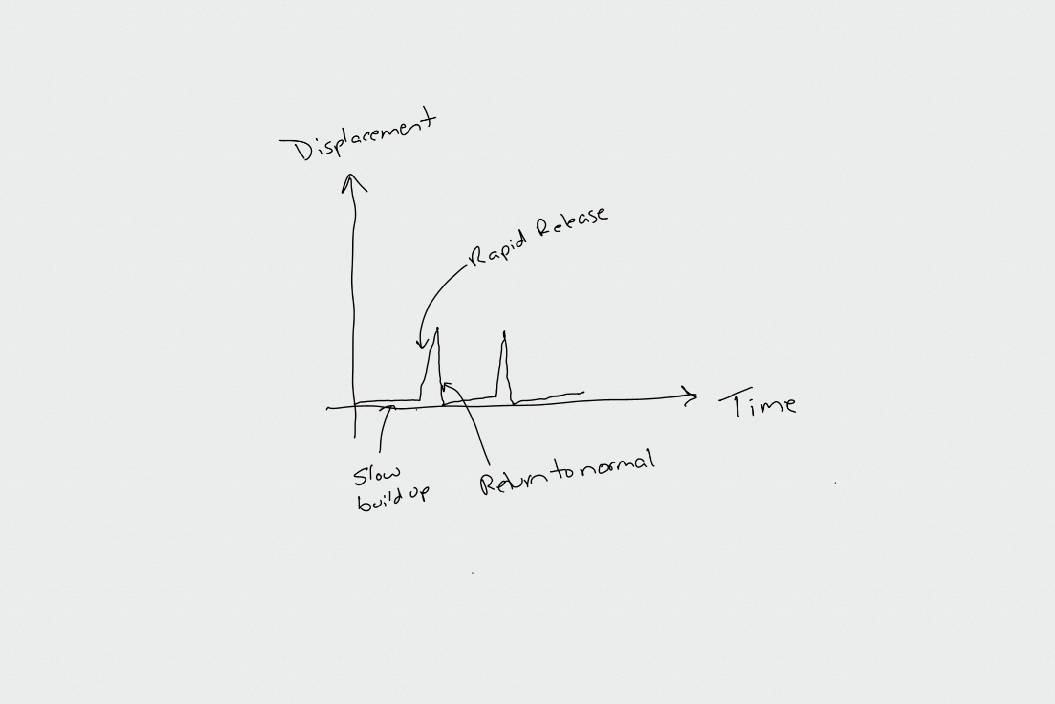
We can pretty easily sketch what a graph capturing the motion of the bucket would look like:
Here, we’ve plotted time on the x-axis and the bucket’s angular displacement from the upright position on the y-axis. For a relatively long time, this displacement changes very little, then, suddenly, there is a rapid change and a rapid reset back to the horizontal position. The whole graph repeats over and over, which we already imagined when we starting thinking “periodic function.” It’s pretty clear however that this isn’t a simple sinusoidal function or any of the other “typical” periodic functions we might talk about in a high school math class. That brings up the question of what the CCSSM intend when they write this:
Interpret functions that arise in applications in terms of the context.
CCSSM HSF.IF.B.4
For a function that models a relationship between two quantities, interpret key features of graphs and tables in terms of the quantities, and sketch graphs showing key features given a verbal description of the relationship. Key features include: intercepts; intervals where the function is increasing, decreasing, positive, or negative; relative maximums and minimums; symmetries; end behavior; and periodicity.*
We didn’t have to look very hard to find an example in an application that doesn’t at all look like the periodic functions they’re studying through the related standards on trigonometric functions. And, here’s where we have an opportunity to really enrich a student’s experience both mathematically and in understanding the applications of mathematics.
If you went no further in class than sketching the behavior of the tipping bucket as we did above and then leading a discussion that drove home the idea that the class of periodic functions is much bigger than the set of trigonometric functions, I’d argue you’ve already done something really important for enhancing their mathematical understanding of functions. You’ve ultimately set them up to better appreciate the magic of Fourier series later on in their studies when they see that all periodic functions can be synthesized from infinite sums of trigonometric functions. (That statement loses some magic for those who think that the only periodic functions are trigonometric functions anyway!)
At the same time, you can also introduce students to the idea of a class of oscillators and help them see the unifying power of mathematics in applications. You’ve likely already showed them multiple systems in the real world that lead to sinusoidal oscillations, now you can introduce the idea of relaxation oscillators and discuss how the tipping bucket is just one particular instance of this class.
Relaxation oscillators are characterized by the behavior we see in the tipping bucket. There is always some slow “build up” phase, a sudden release of energy, and then a return to the start of the build up phase. If you think for a moment, you can probably imagine other instances that you’ve already seen. Here’s another example:
I think it would be fun to challenge your students to go find other instances of systems that demonstrate this slow-build up/rapid release behavior. If you really want to challenge them, you can have them build one of their own:
In our professional development, we talk a lot about the notion of “thought tools” and how to wield them. Today, I’d like to talk a little bit about this idea and see if we can clarify the notion of “thought tool.”
We’ve borrowed the language and the idea of “tools for thinking” or “thought tools” from the philosopher and cognitive scientist Daniel Dennett. (In my humble opinion one of the few living philosophers worth listening too. Nick Bostrom is another.) Dennett lays out the notion of though tools in his book “Intuition Pumps and Other Tools for Thinking” and gave a wonderful talk with the same title at Google.
Both Dennett’s book and his talk do a fantastic job explaining this notion in detail, so here, we’ll just introduce the basic idea and then explore what this has to do with the art of mathematical modeling.
Dennett opens his book with a wonderful quote from one of his former students:
“You can’t do much carpentry with your bare hands and you can’t do much thinking with your bare brain.”
– Bo Dahlbom
He then develops the idea of “tools for thinking” by analogy with ordinary tools. Just as we leverage the power of the hammer or the saw or the chisel to expand our ability to do carpentry and expand the range of carpentry problems we can tackle, Dennett argues that we can and should pay attention to the tools we use for thinking about problems. Just like tools for carpentry, thought tools provide us with the opportunity to tackle harder problems and do a better job with them. So, let’s look at two examples of general thought tools, Sturgeon’s Law and Occam’s Razor.
Sturgeon’s Law is usually expressed as “90% of everything is crap.” That means 90% of papers on molecular biology, 90% of political commentary, and 90% of blog posts on the internet. While the “90” figure isn’t meant to be viewed as a hard and fast quantitative statement, the idea is that in any area, most of what is written or said is, well, crap. The key point is that this statement is also useful for thinking about things. If you’re learning a new subject, don’t waste your time with the 90%, focus on the 10% that’s really good and really important. If you’re a critic, don’t waste our time taking easy shots at the 90%, give us some critical insight into the important 10%. I think this gives you the sense of what a “thought tool” is all about. Generically, it’s a useful way of approaching certain problems.
Occam’s Razor is another such thought tool and likely a familiar one. This one we can state as “Do not multiply entities beyond necessity.” Or, more directly as “Take the simplest theory.” That is, when I flip a switch and a light bulb comes on, I should probably assume an electrical circuit has been closed rather than assume that the switch was a signal for tiny ghosts to light a small fire in the bulb in my lamp. Again, this “thought tool” is a useful way of thinking about and approaching certain problems.
When we think about mathematical modeling, this idea of “thought tools” becomes valuable on two levels. First, the art of mathematical modeling is itself a thought tool. That is, it’s a way of approaching certain types of problems. Just like applying Sturgeon’s Law to the question of what happens when I flip my light switch makes no sense, it’s important to realize and keep in mind that mathematical modeling is a way of approaching certain types of problems. While it’s range of applicability is far greater than that of Sturgeon’s Law or Occam’s Razor, it is still limited, and throwing questions at it for which it’s not equipped is likely to lead to nonsense.
On another level, the idea of thought tools itself gives us a way to think about the teaching and learning of mathematical modeling. Suppose you were observing a philosopher at work and they were asked to choose between the electric circuit or the ghost theory of the light bulb as discussed above. It’s likely they’d, without discussion, simply assume the electric circuit and move on with their lives. It would be up to us to ask “How are you thinking about that?” Such a question would lead us to uncover the idea of Occam’s Razor, which we could then use for ourselves in all sorts of situations. It would then be a heck of a lot easier to teach students about the idea of Occam’s Razor and how to use it than it would be to teach them the answer to every question comparing alternative theories. That is we make more philosophers by teaching students both what to think about and how to do the thinking. But, we as teachers have to carefully observe practitioners and work very hard to understand what is going on with their thinking.
In the same way, we argue that we need to do this with practitioners of the art of mathematical modeling. In a previous post on the modeling cycle, we alluded to this need when we talked about how practitioners don’t really follow a series of steps and how the modeling cycle is only a crude model of the practice. This, in turn, means that there is likely a lot more going on with the mathematical modeler when they are practicing their art. They’re making use of many thought tools that remain hidden unless we work to ferret them out. The modeling cycle gives us some picture, but only in the broadest sense and only of the most obvious of these tools.
As an example, let’s consider “Formulate.” The CCSSM describes this step in their modeling cycle as “formulating a model by creating and selecting geometric, graphical, tabular, algebraic, or statistical representations that describe relationships between the variables.” But, there must be much more to it than that! How exactly do I “select”? Is it like choosing from a menu? Or, is there some other reasoning process involved? How do I “create”? When do I know to “create” versus “select”? Hidden in the practice and in that innocent looking box of “Formulate” there is a heck of a lot more going on.
That’s where this idea of “thought tools” comes back into play. The practicing mathematical modeler has a pretty full toolkit. When they see objects in motion they think “Newton’s Laws” or “F=ma.” When they see a measurable quantity changing with time, they think “conservation law.” And, when they see something in nature choosing a particular shape, they’re likely to be thinking “minimization principle.”
Note that none of these are automatic or inborn and this is where those who would teach mathematical modeling have some work to do. The teacher of mathematical modeling must themselves be a modeler, fill up their toolbox, and be aware enough of what’s in their toolbox that they can identify their thought tools and help equip others in the same way.
As Daniel Dennett says in the opening line to his book – “Thinking is hard.” Similarly, thinking like a mathematical modeler isn’t easy, but thought tools can make the road a little easier to travel.
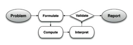
By now, you’re likely familiar with the modeling cycle introduced in the Common Core State Standards.
Today, I want to explore this notion of “modeling cycle” a little bit and urge you to think a little bit differently about this idea. One trend I’ve noticed in the mathematics education community is the deconstruction of this cycle or the listing of the parts like this:
The point is usually made that these are all related to key skills that the mathematical modeler must possess and I wholeheartedly agree with that idea. It’s when the point becomes “these are all key steps in the modeling process” that I start to grow concerned.
Something I’d urge you to keep in mind as you study the teaching and learning of mathematical modeling is that the modeling cycle is not the same thing as mathematical modeling. Now, that sounds a little funny, so let me say it another way. The modeling cycle is simply a model of the process of mathematical modeling and as with all models, we have to be sure not to confuse the model with thing in and of itself! As with all models, the modeling cycle is incomplete, provisional, rests on assumptions that are open to question, and should be used carefully, with all of these points in mind.
If you’ve ever Googled “mathematical modeling cycle” you’ve likely gotten an inkling of this point and encountered other modeling cycles like this one from the Stepping Stones project at Indiana University:
Or this one from Rita Borromeo Ferri:
Hopefully, seeing these different modeling cycles drives home the point that there is no single “modeling cycle” that is any sense “the” modeling cycle, but rather, they are all just different ways to model the process of mathematical modeling.
Recognizing this distinction, or failing to recognize this distinction, has implications for how we teach the art of mathematical modeling. Don’t fall into the trap of believing that the modeling process can be deconstructed into a list of “steps” to follow! Just as when scientists are doing science, they aren’t holding some poster version of the scientific method in their head and going through a linear process, the mathematical modeler isn’t going through a simple checklist either. More likely, they are moving fluidly between steps in a variety of orders, skipping steps, creating new steps, and doing a whole bunch of things that are represented merely as lines connecting steps in a typical modeling cycle.
The primary implication then for teaching and learning is this – don’t attempt to teach the art of mathematical modeling by having your students mechanically plod through the steps in some modeling cycle! Rather, engage them in mathematical modeling through the joint investigation of genuine modeling situations and later use the modeling cycle as a tool to engage them in meta-thinking about what they did and didn’t do during their investigation. Feel free to use whichever modeling cycle best fits your classroom! And, always keep in mind, that the modeling cycle is after all, just a model.
Whenever I’m asked “What’s the most important skill for a mathematical modeler to have?” or “What do you look for in a graduate student?” or “What do you wish every entering university student would have?” my answer is always the same and always one word – curiosity. Now, that could either indicate a stunning lack of imagination on my part or it could indicate that I think this idea of curiosity is pretty important. Today, I’ll try and convince you that it’s the latter of these two, give you an example of what I mean, and along the way, develop some ideas of how to take advantage of some common technology in your classroom.
First, lets talk about this notion of curiosity. In his wonderful book “Curious: The Desire to Know and Why Your Future Depends on It,” Ian Leslie describes two categories of curiosity, distractive curiosity and epistemic curiosity. Distractive curiosity is what keeps us checking email on our phones or refreshing our Twitter feed. It’s the built in craving we all feel for the novel or the new. Easily satisfied, short-lived, and ultimately not very nourishing. Epistemic curiosity is the directed and focused, it’s the form of curiosity that grabs hold of us and and drives us to explore something deeply, with no end in mind, just the desire to really know. When I answer “curiosity” to the inquisitive parent or prospective graduate student, I’m talking about epistemic curiosity, or the unbounded longing to know. I hope you are at least a little convinced that I’m not being lazy in my answers, but rather, can see how a prospective university student, or a graduate student, or any prospective mathematical modeler at any level, would be well-served by having a high level of epistemic curiosity. Maybe next time instead of a one-word answer, I’ll hand the questioner a copy of Leslie’s book.
So, what does this have to do with golf, math, or your classroom? Let me take you along with me on a little investigation into the latest bane of my existence and we’ll explore golf, math, and some ideas for your classroom along the way. As we do so, keep in mind, it’s all driven by curiosity.
As is the case for many occasional golfers, I suffer from the dreaded slice (yes, that’s the latest bane of my existence). The beautiful, satisfying thwack of the ball is spoiled again and again as I watch my initially straightly flying shot arc to the right and end up in the trees or on a good day, the neighboring fairway. Now, a slice is caused by one of two things (or perhaps both), an outside-in swing path or an “open” club-face on contact. I’m fortunate to have golfing buddies who in-between falling over laughing manage to occasionally watch my swing for me and so I’m fairly certain my particular issue is mostly an “open” club face. Striking the ball with an open club face puts a tremendous spin on the ball and quickly the Magnus Effect takes over, causing the curved flight path. In the video below you’ll see a few creative and curious fellows illustrate the Magnus Effect with a basketball and a really high dam.
The Magnus Effect is ultimately an instance of Bernoulli’s Law which you can explore at:
For now, let’s just agree that it would be good if I could put less spin on my golf ball. (But, note how many interesting pathways the curious could follow here!) So, to confirm this “open-club face” hypothesis and to get a handle on just how open it is, I thought it might be useful to be able to video my golf club impacting my ball during my swing. And, this brings me to a neat tool for your classroom – the iPhone 6. Remarkably, the camera on the iPhone 6 is not only of incredible quality, but can do limited high-speed photography as well. To get a grasp on just how cool that is, let me just say that about ten years ago, it cost us more than 10,000 to buy a low-end basic high speed camera for our lab. Yes, that camera could ultimately record much faster, but at an incredibly limited resolution and it’s lower end recording speeds (which were the most useful speeds!) were identical to what the iPhone 6 can now do.
The slow motion setting on the iPhone 6 gives us a frame rate of 240 fps. That is, it will capture 240 frames of video per second. The question then becomes – Is this fast enough to capture my club hitting a ball? Which, of course, brings up the question – How fast is my club head moving when I hit a golf ball? It was at this point in my thinking that I realized I had no idea how fast my club (or any club) was moving. And, this brought to mind the difference between distractive and epistemic curiosity. I could easily Google “How fast does a golf club impact a ball?” I’d get answers that would at least give me a ball park to work in. But, this is where the epistemically curious or the mathematical modeler parts ways with the non-modeler. The mathematical modeler isn’t just seeking an answer, they’re seeking insight. It’s not just a number they want (although that’s part of it), but they want a deeper understanding of whatever it is they are exploring. It’s more work then Googling, but it’s ultimately more valuable as well.
So, let’s do a little quick and dirty mathematical modeling, a “back-of-the-envelope” type analysis. We can get a lower bound on the speed of the club head at impact by idealizing the heck out of the situation. If the lower bound tells us our iPhone 6 can’t capture the impact, then we can move on. If it suggests that it could, we’ll need to improve our model to get a tight lower bound and compare again. We’ll idealize our golfer as a simple pendulum.
Now, suppose we make the assumption that all a golfer does is act like a pendulum, bringing the club head to the top of the travel path and then releases, letting gravity do the rest. Note, we know this is wrong! We know that we are ignoring everything the golfer does to accelerate the club head. That’s why this is a crude lower bound. With these assumptions, we can however quickly and easily compute a lower bound on club speed by using conservation of energy. All of the potential energy at the top of the swing is converted into kinetic energy at the bottom. That is,
(1)
The mass terms cancel, we know the gravitational constant, and if we estimate the initial height of the club head at about 2.5 meters, we get a lower bound for the velocity of our club head of about seven meters per second (15 miles per hour). Those of you who have ever swung a golf club will see instantly that this is very much a crude lower bound. The golfer accelerates the club head through the swing and so we’d expect actual club head speed to be eight or nine times this number. But, we know it should be no slower than this and that’s enough for our calculations today.
So, can our iPhone capture our club head at the moment of contact? To resolve the motion, we can estimate that we’ll need to capture the club head as it moves centimeter by centimeter. If is our frame rate and the velocity of the object we want to capture, then the distance the object travels between frames is simply . Our lower bound on velocity and the known frame rate of 240 fps tells us that our club head is traveling at least 3 centimeters between frames. Knowing that this is a pretty crude lower bound and that the actual club head will be traveling much faster, we can confidently say that it is unlikely that even the really cool iPhone 6 camera will capture this motion. Since it’s always fun (and important) to double-check with reality, here’s a “slo-mo” video of my club hitting a ball.
Sadly, as we predicted, too fast to tell the position of my club face!
But, we’ve discovered a pretty neat new tool that I hope you’ll try out in your classroom. How can you get students playing with “slo-mo,” observing things they haven’t seen before, figuring out how fast things move in the real world, and exploring some cool mathematics along the way? Let us know! Oh, and please don’t take my comments above as being anti-Googling! It’s well worth spending some time poking around on the web searching “math model golf.” You’ll find a lot of neat work that I’m sure will give you other ideas for your classroom. Doug Arnold’s beautiful little paper on “The Science of a Drive” is a great place to start.
Thought I’d share a brief article I wrote for PMENA (Psychology of Mathematics Education, North America, 2014 meeting). This is a pretty good introduction to my perspective on mathematical modeling. – John
Mathematical Modeling – A Practitioner’s Perspective
John A. Pelesko, University of Delaware
Introduction
Having spent the better part of the last twenty-five years engaged in teaching and doing mathematical modeling as an applied mathematician (Pelesko & Bernstein, 2003; Pelesko et.al., 2013), it is hard to overstate the joy I felt upon realizing the special emphasis that the new standards adopted widely across the United States, the Common Core State Standards in Mathematics (National Governors Associate Center for Best Practices & Council of Chief State School Officer, 2010), placed upon modeling. This ascension can be credited in part to the long term efforts of researchers such as Pollak (Pollak 2003, 2012), Lesh (Lesh, 2013), and others who have argued that it is not just applications of mathematics that should be incorporated into the mathematics curriculum at all levels of education, but that the practice of mathematical modeling itself is an essential skill that all students should learn in order to be able to think mathematically in their daily lives, as citizens, and in the workplace (see, e.g., Pollak, 2003). Now that the importance of mathematical modeling is being recognized by the mathematical education community at large, appearing as both a conceptual category and a Standard for Mathematical Practice in the Common Core State Standards in Mathematics (CCSSM), it is necessary that those who do mathematical modeling engage deeply with the K-12 mathematics education community around the issues of teaching and learning the practice. It is important to note that mathematical modeling is practiced far and wide – across the natural sciences, engineering, business, economics, the social sciences, and in almost every area of study in one form or another. Hence, the set of stakeholders in this conversation is large, and we should be careful not to substitute any one practitioner’s perspective for the whole. Nevertheless, in an attempt to contribute to this conversation, here I provide one practitioner’s perspective.
What is Mathematical Modeling?
Given the lack of attention that has been paid to mathematical modeling in the US educational system, especially in mathematics teacher education programs (Newton et.al., 2014), it is not hard to imagine that many mathematics educators upon reading the CCSSM found themselves asking this question. The brief description of mathematical modeling found in the CCSSM (pages 72-73) and the fact that this description first appears within the high school standards likely adds to this confusion. Further confusion is likely to occur as educators digest the Next Generation Science Standards (NGSS Lead States, 2013), which make use of the term “model” both in and out of the context of “mathematical model.”
To address the question “What is mathematical modeling?” it is then perhaps useful to first consider the question “What is modeling?” My answer? Modeling is the art or the process of constructing models of a system that exists as part of reality. By “model,” I mean a representation of the thing that is not the thing in and of itself. The model captures, simulates, or represents selected features or behaviors of the thing without being the thing. By “mathematical model” I mean a model or a representation that is constructed purely from mathematical objects. So, mathematical modeling is the art or process of constructing a mathematical model. That is, mathematical modeling is the art or process of constructing a mathematical representation of reality that captures, simulates, or represents selected features or behaviors of that aspect of reality being modeled.
Now, we should note that mathematical models have a special place in the hierarchy of models in that they have both predictive and epistemological value. The epistemological value is a consequence of the idea that mathematicalmodeling is a way of knowing. The predictive value of a mathematical model gives mathematical models a special place in “science,” loosely and broadly defined, in that a mathematical model can take the place of direct ways of knowing, in other words, experiment. A good mathematical model is both an instrument, like a microscope or a telescope, allowing us to see things previously hidden, and a predictive tool allowing us to understand what we will see next.
Note that an especially “good” mathematical model, that is, one with a high level of predictive success, often ceases to be thought of as “just a model.” Rather, it attains a different status in the scientific community. We don’t say “Newton’s mathematical model of mechanics,” rather we say “Newton’s Laws.” We don’t say “Schrodinger’s model of the subatomic world,” rather we say “Quantum Mechanics” or the “Schrodinger Equation.” Yet, each of these examples is, in fact, a mathematical model of the thing, and not the thing in and of itself. These examples have attained the highest possible level of epistemological value. They have become the way of knowing, understanding, describing, and talking about their subjects.
Now, we have diverged into abstract territory and we do not want to leave the reader with the impression that mathematical modeling is hard, something to be left to the Newtons and Schrodingers of the world. Rather, we hope the reader is left with the impression that mathematical modeling is exceedingly useful and that by helping our students master this practice, we will be adding a tool to their mental toolkit that will serve them well, no matter what their future plans.
Thought Tools for Modeling
The question then becomes: How exactly does someone become a proficient mathematical modeler? In the United States, as evidenced by textbook after textbook on mathematical modeling (Pelesko & Bernstein, 2003)[1], the answer has been “Modeling can’t be taught, it can only be caught.” Here, I take a different perspective and argue that it is useful to think of the mathematical modeler as having discrete “thought tools,” each of which can be discovered and taught. As a consequence, we see that many “modeling cycles” unintentionally hide much of the real work of mathematical modeling.
We borrow the term “thought tools” and this framework for meta-thinking from the philosopher and cognitive scientist, Daniel Dennett. In (Dennett, 2013) he quotes his students as having made the observation that “Just as you cannot do much carpentry with your bare hands, there is not much thinking you can do with your bare brain.” Dennett then proceeds by analogy with saws, hammers, and screwdrivers, to introduce thought tools of informal logic such as reductio ad absurdum, Occam’s razor, and Sturgeon’s Law[2]. Applying this notion of thought tools to the mathematical modeler, we argue that they must possess a set of thought tools that lie in three different categories: Mathematical Thought Tools, Observational Thought Tools, and Translational Thought Tools.
Mathematical Thought Tools are those tools we attempt to add to our student’s toolkits when we teach mathematics. These include notions such as algebraic thinking, the principle of induction, the pigeonhole principle, and any tool that lets students think about and do mathematics. Note that these thought tools are directed at mathematics and their utility is generally tied to thinking in the mathematical domain.
Observational Thought Tools are those tools we typically think of as being used by “scientists.” These include the ability to think in terms of cause and effect, to observe spatial and temporal patterns in the real world, and to look deeply at reality. Note that these thought tools are directed at the real world and their utility is generally tied to thinking in the domain of the real world[3].
Translational Thought Tools are those tools that allow the mathematical modeler to take questions formed in the observational domain and translate them into the mathematical domain and translate answers and new questions uncovered in the mathematical domain back again to the observational domain. These include knowledge of conservation laws, physical laws, and the assumptions that must be made about reality in order to formulate a mathematical model. Note that these thought tools are directed both toward reality and toward mathematics. Their utility lies in their usefulness in translating between these two domains.
In a typical “modeling cycle,” such as appears in the CCSSM, one moves from the “real world” or the “problem” to the “formulation” via a single small arrow. Buried in this small arrow is the use of Observational and Translational Thought Tools. The remainder of the cycle, up to the point of comparing results with reality, generally relies purely upon Mathematical Thought Tools. While we can argue over whether or not we are properly equipping our students with the Mathematical Thought Tools they will need in their journeys around the modeling cycle, I would argue that generally we pay little attention to the Observational and Translational Thought Tools they will need to begin their journey. Identifying, unpacking, and learning how to equip our students with these sets of tools is an essential step in learning how to teach mathematical modeling.
As an example of how the mathematical modeler wields these tools, I ask the reader to imagine drops of morning dew on a spider web. The scientist, using their observational tools, notices these droplets and wonders why they are all roughly the same size. The mathematical modeler recalls that nature acts economically and often in a way that minimizes some quantity. They cast forth a hypothesis that here, nature is acting to minimize surface area, and that leads the dew to break into droplets of nearly uniform size. They recast this observation and hypothesis into mathematical terms, already anticipating the mathematics from the presence of the notion of “minimizes” and wield their Mathematical Thought Tools to predict the size of the droplets given the presence of the dew. Comparing their predicted size with the size of actual droplets, they refine and perfect their model, and have acquired an understanding of any droplets on any spider web at any point in time.
Conclusion
Mathematical modeling is a practice worth sharing and teaching. Mathematical modeling is a powerful way of knowing the world, and it can be taught rather than simply caught. In the United States, we have much work to do in order to bring this new toolkit to our students. It will take the efforts not only of mathematics educators and applied mathematicians, but of mathematical modelers of every stripe in order to do so. Here, I have sketched out one avenue of approach that in many ways parallels recent work in unpacking the thought processes behind mathematical proof (Cirillo, 2014). A similar effort to identify and unpack the thought tools of the mathematical modeler holds the promise of helping us train a wide range of students in the art of mathematical modeling.
References
Pelesko, J. A., & Bernstein, D. H. (2003). Modeling MEMS and NEMS. Boca Raton, FL: Chapman & Hall/CRC.
Pelesko, J.A., Cai, J., & Rossi, L.F. (2013). Modeling modeling: Developing habits of mathematical minds. In A. Damlanian, J.F. Rodrigues & R. Straber (Eds.), Educational Interfaces between Mathematics and Industry (pp. 237-246). New York: Springer.
Pollak, H. O. (2003). A history of the teaching of modeling. In G. M. A. Stanic & J. Kilpatrick (Eds.), A history of school mathematics (pp. 647-669). Reston, VA: NCTM.
Pollak, H. O. (2012). Introduction: What is mathematical modeling? In H. Gould, D. R. Murray & A. Sanfratello (Eds.), Mathematical modeling handbook (pp. viii-xi). Bedford, MA: The Consortium for Mathematics and Its Applications.
Lesh, R., & Fennewald, T. (2013). Introduction to Part I Modeling: What is it? Why do it? In R. Lesh, P.L. Galbraith, C.R. Haines & A. Hurford (Eds.), Modeling students’ mathematical modeling competencies (pp. 5-10). NY: Springer.
Newton, J., Maeda, Y., Senk, S. L., Alexander, V. (2014). How well are secondary mathematics teacher education programs aligned with the recommendations made in MET II? Notices of the American Mathematical Society, 61(3), 292-5.
National Governors Association Center for Best Practices & Council of Chief State School Officers. (2010). Common Core State Standards for Mathematics. Retrieved from http://www.corestandards.org/math.
NGSS Lead States (2013). Next generation science standards. Achieve, Inc. (on behalf of the twenty-six states and partners that collaborated on the NGSS).
Dennett, D.C. (2013). Intuition Pumps and Other Tools for Thinking. New York: W.W. Norton & Company.
Borromeo Ferri, R. (2007). Personal experiences and extra-mathematical knowledge as an influence factor on modelling routes of pupils. Paper presented at the Fifth Congress of the European Society for Research in Mathematics Education (CERME 5) Cyprus, Greece.
Cirillo, M. (2014). Supporting the introduction to formal proof. In P. Liljedahl (Ed.), Proceedings of the Psychology of Mathematics Education International Conference. Vancouver, Canada.
[1] I am as guilty of this approach as the majority of authors of textbooks on mathematical modeling.
[2] Reductio ad absurdum is the form of argument which shows that a statement is true by reducing its’ opposite to an absurd conclusion and is closely related to proof by contradiction. Occam’s Razor is the principle that the simplest explanation is the most likely. Sturgeon’s Law is stated succinctly as “Ninety percent of everything is crap.”
[3] Note again that Observational Thought Tools require real-world experience. This is closely linked to the idea of “Extra-Mathematical Knowledge” being necessary for doing mathematical modeling. (See Borromeo Ferri, 2007)
One of my favorite ways to teach mathematical modeling is through the use of hands-on activities. Often, these are “toy models” of bigger, more difficult to grasp, physical systems. Lately, I’ve been exploring the use of inexpensive, open-source sensors for the Arduino as a vehicle for getting real data from toy models. An Arduino based system allows for the integration of basic electronics, computer science, and programming into the exercise. I’d like to develop projects or systems that aid in the teaching of mathematical modeling, but also tie mathematical modeling together with the sciences in ways that can encourage a more interdisciplinary approach to teaching mathematical modeling.
My ultimate goal is to continue to develop projects aimed at supporting the teaching and learning of mathematical modeling, but that have a hands-on component. A general project structure:
1. The “big problem,” that is, the broad real-world phenomena or scenario.
2. A related analogical model system that is easy to experiment with and observe. (“Toy model.”)
3. A quantity of relevance that can easily be measured in the analogical model system via an Arduino sensor.
Project #1: The Great Lakes Problem
In this project, we’ve posed the problem of understanding pollution in the Great Lakes. This is a relevant problem, easily transferable to local contexts, a challenging problem, yet “low floor/high ceiling” mathematically, and can easily illustrate the full modeling cycle. I’ve used this many times in undergraduate courses on mathematical modeling, but never with a hands-on component. This past week at our summer New Normal academy on mathematical modeling, we tried the hands-on version.
The “Toy Model”
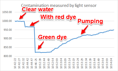
For an analogical model of the Great Lakes problem, we consider a simple system of three containers. The first container has “clean” water. The second “polluted” water dyed with food coloring, and the third is empty. Water flows from container one to container two and out of container two at the same rate. This provides a physical/analogical model of the natural cleansing of a lake under the assumption that all future pollution is stopped. A key question to investigate would be “How long would it take for the lake to reach x% polluted under this scheme?” To measure pollution levels in the system, we use a light sensor and an LED light array. The LED’s are arranged to pass through the “lake” and impinge on the sensor. As pollution levels drop, opacity of the water increases and the light sensor reacts accordingly. Sensor data can be recorded in real-time at any desired time interval using the Arduino. Here is our system:
We began with some basic tests. Light sensor readings through a clear container, no water.
With LED flashlight on opposite side, we get max reading ~995 to ~1000. Next, fill with water and see reading. No apparent change! Good.
Now, the key test, dye the water and see if we get a reduced reading. Use standard liquid red food coloring. 10 drops. Well stirred. Good! We get a change to about 967. Would like a more dramatic change, so add 5 drops of green. Great, now goes to about 823 and water appears black.
So, we have proof of concept, we can measure “contamination” in water using a simple light sensor.
Now, try pumping system and see if we can record changes. Both pumps set to lowest possible rate. We’re using a free plug-in for Arduino and Excel that lets us capture the data in real-time. Works perfectly!
The plot above shows time vs. the light sensor reading.
What would a simple analytic model of this system look like? Identify key variables:
C(t) = Concentration of pollution in Tank #2 at time t.
V = Volume of water in Tank #2.
R = Outflow rate (assumed equal to inflow rate)
dt = A small time interval
Units:
[C(t)] = mass/L^3
[V] = L^3
[R] = L^3/time
[t] = time
[dt] = time
Basic conservation law:
C(t+dt)V = C(t)V – C(t)Rdt
That is:
Total pollution in tank at time t+dt = Total pollution in tank at time t – Amount of pollution that flowed out of the tank
Note, a quick rearrangement yields
(C(t+dt)-C(t))/dt = – (R/V) C(t)
Of course, a limit as dt tends to zero gives the standard first order ODE for exponential decay. What is of most note here is the ratio that controls the rate of decay, namely R/V. Perfectly intuitive in retrospect, this just relates how much stuff flows out to the entire volume. For the data set above, fitting tells us this ratio is about -0.015. We should ask: does the pump flow rate compared to the volume in the tank come close to 0.015? That is, would be good to do those actual measurements for our system. (Didn’t do that yet!)
Note also that one need not go to an ODE here, but could just compute on the model above. In reality, it is just a one-step Euler method applied to the ODE. What questions can this model answer?
– How long does it take for the lake to reach a given pollution level under this scenario?
One can then modify this model to include sources of pollution, coupling between lakes, etc. Another idea would be to do the case where pollution sediments out over time.
Just some random thoughts on a first attempt to use an Arduino with a toy model to do a little teaching and learning of mathematical modeling… Went well with our New Normal academy. Looking forward to developing more such activities and trying them out.


![[x]](http://modelwithmathematics.com/wp-content/ql-cache/quicklatex.com-47d8ad41e1376ae731e01d55fa1edc53_l3.png "Rendered by QuickLaTeX.com") you should read this as “the units of x.” That is, square brackets around a quantity indicate that we are looking at that quantities’ units rather than the quantity itself. So, returning to Taylor’s four quantities of interest, we can write:
you should read this as “the units of x.” That is, square brackets around a quantity indicate that we are looking at that quantities’ units rather than the quantity itself. So, returning to Taylor’s four quantities of interest, we can write:![[\rho] = \frac{M}{L^3}](http://modelwithmathematics.com/wp-content/ql-cache/quicklatex.com-f201ee75364646f478c411a8d1ef0e87_l3.png "Rendered by QuickLaTeX.com")
![[R] = L](http://modelwithmathematics.com/wp-content/ql-cache/quicklatex.com-d1a52c47bf0dabf262ebb1e9fb1ce26c_l3.png "Rendered by QuickLaTeX.com")
![[E] = \frac{M L^2}{T^2}](http://modelwithmathematics.com/wp-content/ql-cache/quicklatex.com-e50e1ec121cbff5d13879a3bdb18559c_l3.png "Rendered by QuickLaTeX.com")
![[t] = T](http://modelwithmathematics.com/wp-content/ql-cache/quicklatex.com-5ced0e7d6bebf89bf48fd4a28723afd4_l3.png "Rendered by QuickLaTeX.com")
 indicates mass,
  indicates length, and
  indicates time. We don’t really care right now whether we use seconds or hours. We do care that our base units are irreducible. That is, none of these units could be expressed in terms of some combination of the other units we’re using. We couldn’t, for example, express time as some combination of length and mass.
 ,
,  , and
, and  are not yet known. But, Taylor did know that his assumed functional form had to be dimensionally consistent. That is, the units in the expression must balance in order for this to make sense! The radius of the blast,
  , has units of length. This means that the powers of the terms on the right must be such that the units combine to reduce purely to length. This, we can express mathematically! Using our bracket notation:
![[R] = L = [E]^x [\rho]^y [t]^z](http://modelwithmathematics.com/wp-content/ql-cache/quicklatex.com-d8fe1fb561192f9d37cdffb7aaadf903_l3.png "Rendered by QuickLaTeX.com")
![[R] = L = M^{x+y} L^{2x-3y} T^{-2x+z}](http://modelwithmathematics.com/wp-content/ql-cache/quicklatex.com-c681c89fb492b2654a328914cc997c42_l3.png "Rendered by QuickLaTeX.com")


 , and from the Life magazine photo he knew the radius of the blast,
  . That meant he knew everything in this expression except for
  , which he was trying to find, and could now solve for
 10,000 to buy a low-end basic high speed camera for our lab. Yes, that camera could ultimately record much faster, but at an incredibly limited resolution and it’s lower end recording speeds (which were the most useful speeds!) were identical to what the iPhone 6 can now do.
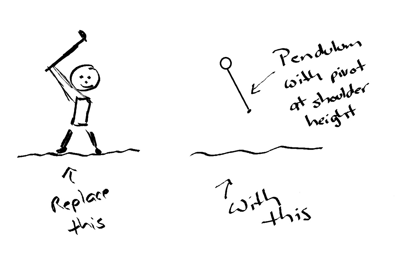

 is our frame rate and
  the velocity of the object we want to capture, then the distance the object travels between frames is simply
  . Our lower bound on velocity and the known frame rate of 240 fps tells us that our club head is traveling at least 3 centimeters between frames. Knowing that this is a pretty crude lower bound and that the actual club head will be traveling much faster, we can confidently say that it is unlikely that even the really cool iPhone 6 camera will capture this motion. Since it’s always fun (and important) to double-check with reality, here’s a “slo-mo” video of my club hitting a ball.
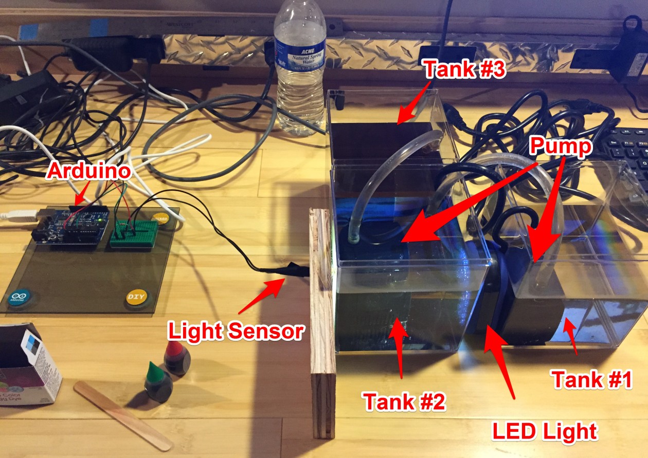
.png)