In the CCSSM several of the “starred” high school standards relate to quantitative reasoning and using units to solve problems:
Reason quantitatively and use units to solve problems.
CCSS.MATH.CONTENT.HSN.Q.A.1
Use units as a way to understand problems and to guide the solution of multi-step problems; choose and interpret units consistently in formulas; choose and interpret the scale and the origin in graphs and data displays.CCSS.MATH.CONTENT.HSN.Q.A.2
Define appropriate quantities for the purpose of descriptive modeling.CCSS.MATH.CONTENT.HSN.Q.A.3
Choose a level of accuracy appropriate to limitations on measurement when reporting quantities.Modeling Standards: Modeling is best interpreted not as a collection of isolated topics but rather in relation to other standards. Making mathematical models is a Standard for Mathematical Practice, and specific modeling standards appears throughout the high school standards indicated by a star symbol (*).
By the presence of the star, as the footnote in the CCSSM indicates, we know that this particular set of standards is of special importance to the practice standard, “Model with mathematics.” In any modeling process, paying attention to units, constantly checking that model equations are consistent in terms of units, and defining appropriate quantities are all crucial skills. Today, I’d like to explore the related skill of “dimensional analysis.” This is a skill that is pretty typically in the toolbox of the practicing mathematical modeler, yet, hasn’t seemed to make its way to the high school classroom.
It’s easiest to illustrate the idea of “dimensional analysis” with a story and as with many stories around mathematical modeling, this one revolves around the great G.I. Taylor. Taylor was an incredibly prolific physicist and mathematician (1865-1975) the bulk of whose work was in fluid dynamics, but who possessed a wide-ranging mind, and made fundamental contributions to multiple areas of study. The “FRS” at the end of his name and the “Sir” at the beginning might give you some idea of the impact of his work. His biographer, George Batchelor, himself a very notable scientist, described Taylor as “one of the most notable scientists of this (the 20th) century.”
This particular story about Taylor takes place in 1950, shortly after the development of the first atomic bomb. That year, Life magazine published a photo essay featuring high-speed photographs of the first man-made atomic explosion at the “Trinity” site in New Mexico. Here’s one of the photographs that Taylor would have seen in the Life magazine article:
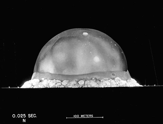
Now, notice the two pieces of data on this photograph. The first is a time stamp which tells the number of seconds elapsed since the explosion (0.025 seconds). The second is a scale bar that allows anyone with a ruler to determine the blast radius at that instant in time. Using just this data Taylor estimated the yield of the explosion, or the energy released, to be 22 kilotons (of TNT). The highly classified official estimate of the yield was 20 kilotons. Taylor got within 10% of the highly classified estimate with only a photograph from Life magazine at his disposal!
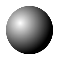
How did he manage this? Well, Taylor used the tool of dimensional analysis. Let’s see exactly how he reasoned. Taylor began with a simplifying assumption. He assumed that the energy was released in a small spherical area and that the shockwave we see stays spherical. That is, he replaced the picture above, which is more hemispherical, with:
Next, he identified four quantities of interest:


Now, Taylor knew the units of each of these quantities, but let’s make them explicit here. To do this, we’ll introduce a piece of notation that’s very handy when doing dimensional analysis, the “square brackets.” Whenever we write ![[x]](http://modelwithmathematics.com/wp-content/ql-cache/quicklatex.com-47d8ad41e1376ae731e01d55fa1edc53_l3.png "Rendered by QuickLaTeX.com") you should read this as “the units of x.” That is, square brackets around a quantity indicate that we are looking at that quantities’ units rather than the quantity itself. So, returning to Taylor’s four quantities of interest, we can write:
you should read this as “the units of x.” That is, square brackets around a quantity indicate that we are looking at that quantities’ units rather than the quantity itself. So, returning to Taylor’s four quantities of interest, we can write:
![[\rho] = \frac{M}{L^3}](http://modelwithmathematics.com/wp-content/ql-cache/quicklatex.com-f201ee75364646f478c411a8d1ef0e87_l3.png "Rendered by QuickLaTeX.com")
![[R] = L](http://modelwithmathematics.com/wp-content/ql-cache/quicklatex.com-d1a52c47bf0dabf262ebb1e9fb1ce26c_l3.png "Rendered by QuickLaTeX.com")
![[E] = \frac{M L^2}{T^2}](http://modelwithmathematics.com/wp-content/ql-cache/quicklatex.com-e50e1ec121cbff5d13879a3bdb18559c_l3.png "Rendered by QuickLaTeX.com")
![[t] = T](http://modelwithmathematics.com/wp-content/ql-cache/quicklatex.com-5ced0e7d6bebf89bf48fd4a28723afd4_l3.png "Rendered by QuickLaTeX.com")
Notice that we haven’t bothered to pick a particular system of units. We’re not really worried whether we’re using centimeters, grams, and seconds or kilometers, grams, and seconds. What we’re worried about here is just that we’re expressing these in terms of fundamental units. That is, we are at the “atomistic” level of our units. We’re not using derived units like Amperes or Newtons. Rather, we’re being careful to capture the basic units or each of our quantities. Here,  indicates mass,
  indicates length, and
  indicates time. We don’t really care right now whether we use seconds or hours. We do care that our base units are irreducible. That is, none of these units could be expressed in terms of some combination of the other units we’re using. We couldn’t, for example, express time as some combination of length and mass.
Now that we have our units cleared-up, let’s move along with Taylor. His next step was to assume a functional relationship of a particular form between his four quantities. He imagined that the blast radius could be determined if he knew the energy released in the blast, the density of the surrounding air, and the time elapsed since the explosion. So, he wrote the radius as a product of powers of these three quantities. This is the key step in dimensional analysis. It’s supported by what is known as the “Buckingham Pi Theorem” which formalizes the informal process we’ve described here. But, proceeding informally, here’s what Taylor wrote:

The powers,  ,
,  , and
, and  are not yet known. But, Taylor did know that his assumed functional form had to be dimensionally consistent. That is, the units in the expression must balance in order for this to make sense! The radius of the blast,
  , has units of length. This means that the powers of the terms on the right must be such that the units combine to reduce purely to length. This, we can express mathematically! Using our bracket notation:
![[R] = L = [E]^x [\rho]^y [t]^z](http://modelwithmathematics.com/wp-content/ql-cache/quicklatex.com-d8fe1fb561192f9d37cdffb7aaadf903_l3.png "Rendered by QuickLaTeX.com")
Or,
![[R] = L = M^{x+y} L^{2x-3y} T^{-2x+z}](http://modelwithmathematics.com/wp-content/ql-cache/quicklatex.com-c681c89fb492b2654a328914cc997c42_l3.png "Rendered by QuickLaTeX.com")
Of course, the only way for the units on the right to reduce to length alone is if:


Ah, we’re at the “solve systems of equations” line in the high school standards! So, I’ll let you do the algebra, and just note that solving this system told Taylor that:

Taylor knew the density of air,  , and from the Life magazine photo he knew the radius of the blast, , at a particular time,
  . That meant he knew everything in this expression except for
  , which he was trying to find, and could now solve for . That’s how Taylor obtained his estimate of 22 kilotons.
I hope this gives you some sense of the power of this approach and also helps you see dimensional analysis as a relatively simple to use tool in the modeler’s toolbox. If you want to explore this further, just let me know. In the meantime, I’ll leave you with a video I often share with my students. I ask them to use this video and dimensional analysis to estimate the gravitational acceleration on the moon.
– John