In his interesting recent book, Average is Over, economist Tyler Cowan spends considerable time discussing and analyzing the phenomena of “freestyle chess.” While Cowan is interested in the future of the economy, the future of work, and the impact of technology on the workplace, aspects of the freestyle chess movement struck me as a good analog for how mathematical modeling activities should play out in the classroom or in the workplace. So, today, I’d like to explore that notion a bit and introduce the idea of “freestyle math.”

Chess, of course, developed as a competitive game between two players. The relative simplicity of the rules and the absence of chance as an aspect of the game combined with the deep complexity and tremendous variety of possible play has made chess an enduring pastime played by millions for about 1400 years. For most of that time, the standard of play was human vs. human, with exceptionally talented humans becoming “grandmasters,” people who could play at extraordinarily high levels.

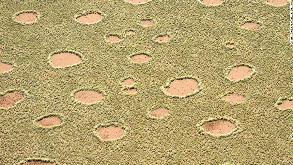
In the 1950’s, things began to change. Alan Turing, who we discussed in a previous post on pattern formation, realized that a computer could in principle be programmed to play chess. Turing even developed strategies for such a program and wrote chess-playing code long before the computer hardware side of the world was developed enough to execute such code. However, before long, the hardware side of the world was up to speed and by the 1970’s one could purchase a dedicated chess-playing computer that looked like this:

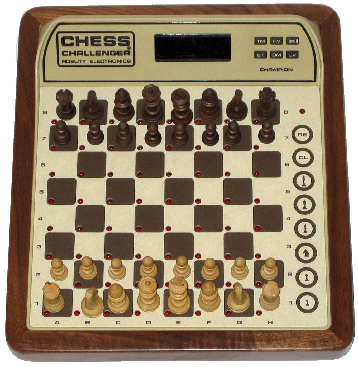
I recall an uncle of mine owning one of these early machines and I recall being amazed that the computer could pretty handily beat everyone I knew. But, at that time, at least, really good humans were still far better than the best chess playing machines. This too changed rapidly and in 1997, a computer called Deep Blue, developed by IBM, beat the reigning world chess champion, Gary Kasparov, 3 1/2 to 2 1/2 in a six game match. (Note that 1/2 points are awarded to each side in a draw.)

In the last eighteen years, computers have only gotten better at chess and humans, well, haven’t. Today’s most talented players don’t stand a chance against a good chess program and a good chess program can now be a single app on the phone in your pocket. However, shortly after losing to Deep Blue, Kasparov asked an interesting question – What would happen if instead of human vs. human or man vs. machine the competition were man + machine vs. man + machine. The new competitive sport of “freestyle chess” was born soon thereafter.

In this incarnation, chess is a team sport, where members of the team may be computer programs. In fact, in freestyle chess pretty much anything goes with Kasparov having remarked “Even if they were assisted by the devil, that would probably be covered by the rules.” And, in freestyle chess, something remarkable happened. Human-machine teams could defeat a single top-ranked chess playing computer program. The level of chess played by these man/machine hybrid teams was now higher than that played by either man or machine alone in the past.

Cowan describes freestyle chess matches as a being like a beehive of frenetic activity with human teams scurrying from computer to computer, combining, and analyzing suggested moves from multiple analyses before making a final decision. He also notes, interestingly, that the best freestyle teams are not necessarily made up of top chess players working with top chess computer programs. Rather, a strong freestyle team needs humans with a very different skill set. Yes, they have to understand chess and the basic elements of play, but they also need to understand computer programs, how they work, what their limitations are, what their strengths are, and how to combine the brute-force “number crunching” approach of computers effectively with human intuition.

As I read Cowan’s description of freestyle chess, I was struck by how similar the activity he described is to the activity of an effective student team working on a mathematical modeling investigation. So, I’d like to encourage you to think of mathematical modeling in your classroom as “freestyle math” and I’d like to explore for a moment some of the characteristics of what that might look like. I’m encouraging you to think of “freestyle math” in this “anything goes” sort of mindset. That is, students should be free to tap into the internet, simulation, textbooks, friends, etc., without bound. The focus should be on the goal of understanding the phenomenon they are investigating and in how one gets there, anything should be fair game. So, here are five characteristics of freestyle chess that I believe map in a one-to-one fashion to freestyle mathematical modeling:

The humans know something, but might not be super-experts

In freestyle chess, the human members of the team are not necessarily grandmaster level chess players or even master level chess players. But, at the same time, they know the rules of the game, have an understanding of strategy, and generally play as well as a decent club player (someone who plays regularly). On a modeling group in the high school classroom you want your “players” to have a roughly similar level of expertise in mathematics and have some expertise in the application area they are investigating. You don’t need a team full of math-whizzes, but you do need your students to take ownership of the mathematics, have a comfort with using mathematics, and be able to know what they need to learn.

Collaboration is key

As in freestyle chess, in freestyle math, the ability to collaborate effectively, both with other humans and with computers is a key skill. The ability to work with a diverse team is important and students also need to know how and when to use technology in their investigations. This means our students need to know when to “Google” and when to think. They need to know when to analyze with pencil and paper and when to turn to the computer.

The humans understand the strengths and limitations of computers

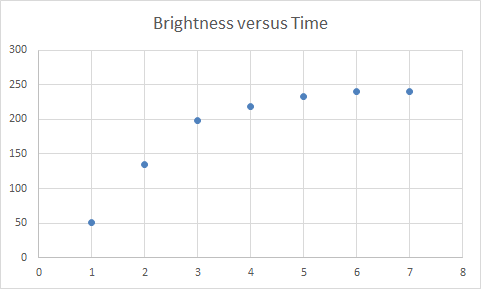
An essential skill of freestyle chess players is knowing both the strengths of various computer programs and the limitations of various computer programs. This is at least as important of a skill for mathematical modelers to possess. They should know to turn to the computer to fit a curve to a data set consisting of even a mildly large number of data points. At the same time, they should know what the computer is doing when it is fitting that curve, what assumptions they are making when they take that curve as being predictive, and exactly where the limitations are in what the computer is telling them. I can’t emphasize this one enough – to use a tool effectively you have to know both what it is good for and what it isn’t.

The humans are able to tap into and filter vast quantities of information

In freestyle chess, humans also bring the ability to both gather vast quantities of information and to filter this information. Freestyle math needs the same skill. Even a discerning Google search about a real-world scenario that students might investigate will return hundreds of thousands of links. Students need to be able to quickly and efficiently zoom in on the relevant information and know what information to trust and what to ignore. At the same time, a simple computer simulation can also quickly return reams of data. Students need to know how to organize this information, how to visualize this information, and again pick out what is relevant and what isn’t.

The humans supply creativity and intuition

Humans clearly bring both creativity and intuition to the table and both of these skills are required in abundance in freestyle chess and in freestyle math. In mathematical modeling, decisions, false starts, retrenchments, intuition, and creativity are the norm. Students need to be able to offload to a computer the things it does best and bring to the table the sorts of creative approaches and intuition that they do best.

As you work to engage your students in the practice of mathematical modeling I’d encourage you to think “freestyle math” and look to freestyle chess as a model for what open collaboration between people and between man and machine can produce. I’d also encourage you to think about the skills that such activities demand that go beyond the simple mastery of mathematical procedures, and how freestyle math demands a deep understanding of concepts and the ability to integrate that knowledge in the pursuit of understanding the world.

John

Often in mathematics, and certainly often in mathematics class, we think in terms of direct problems.  That is, we’re given something to “solve,” we’re required to find a path to a “solution,” and that’s where we end up. For example, we might be asked to find the solutions of the following equation

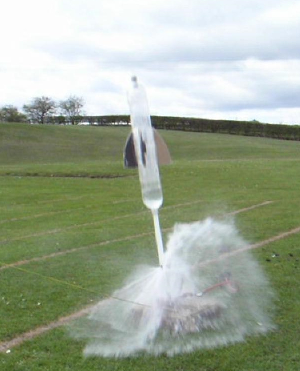
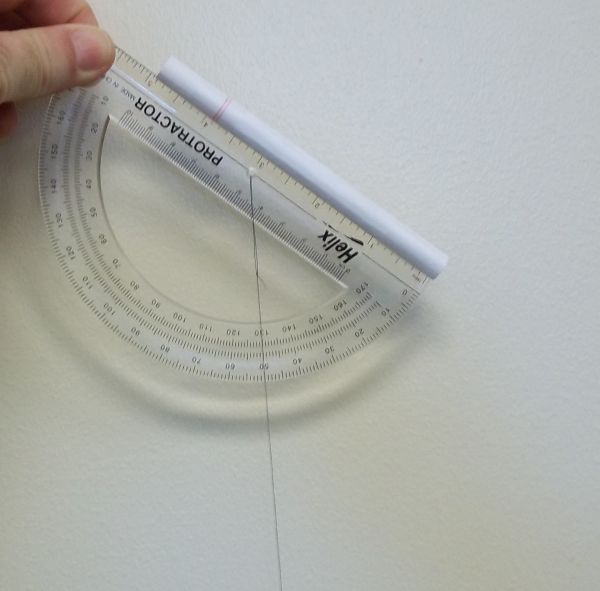
and we proceed by using the quadratic equation or completing the square or some such method, and arrive at values for . If we think of this in terms of applications, we often pose direct problems as well. Here, for example, we might say, suppose we drop a ball from a height , we assume air resistance is negligible, how fast is the ball traveling when the ball hits the ground? Or perhaps, how long will it take the ball to hit the ground?

But, often, in the real world, our problems aren’t formulated like this. Rather, we’re faced with problems that are posed the other way around. That is we’re faced with what are called inverse problems.  In these problems, what we’re given is the solution and what we have to do is figure out where it came from. You’re likely familiar with such problems, but perhaps haven’t thought of them in this way before. One common example is the “sonar problem” or the problem of echolocation. If I’m a bat, what I do is make a noise, and then listen for the reflected sounds that come back to me. What I then try and do is figure out the direction, location, and perhaps shape, of the objects in the environment that caused the particular patterns of reflected sounds that I heard. That is, I’m given the solution, i.e. the reflected sounds I measured, and have to figure out the problem, i.e. what pattern and shape of objects in the environment would cause that set of reflected sounds?

Such problems are an important class of problems that the mathematical modeler must be equipped to deal with. And, such problems, can be a source of challenging and engaging problems for students learning the art of mathematical modeling. Today, I’d like to explore a few simple versions of such problems and how you might use them in your classroom.

One of my favorites is a problem that was posed by Isaac Newton in Universal Arithmetik and was discussed by Groetsch in his text Inverse Problems: Activities for Undergraduates. Newton posed the problem like this:

A Stone falling down into a Well, from the Sound of the Stone striking the bottom, to Determine the Depth of the Well.

The unusual capitalization is Newton’s and apparently the style of the time was to state commands rather than pose questions. Today, we might state the problem as:

Can we determine the depth of a well by dropping a stone into the well and listening for the sound of the stone striking the bottom?

Why is this an inverse problem? Well, what we’re asked to do here is to take information we obtain at the end of a process, i.e. the time interval between us releasing the stone and it us hearing the stone strike the bottom of the well, and to infer how the stone must have traveled and from this deduce the depth of the well.

This particular inverse problem can be approached by solving the direct problem, which requires us to build a mathematical model of the time which elapses between the release of the stone and us hearing the sound of the stone striking the bottom of the well. We can imagine that we release the stone and start a stopwatch at the same instant. When we hear the sound, we stop our stopwatch and call that elapsed time, . Further, we can suppose that can be divided into two parts, the time it takes the stone to fall, , and the time it takes the sound to travel back up the well, . Our measured time is then the sum of these two:

Our job is then to build a model of the fall and the travel of the sound that lets us express and in terms of the depth of the well, . It’s worth noting that both modeling the fall and understanding the fact that sound travels at a finite speed fall within the scope of the NGSS standards and so, should be within reach of the high school classroom. I’ll skip the details here, but you should be able to arrive at an expression that looks like:

Here, is the gravitational acceleration and is the speed of sound in air. A quick plot of as a function of yields: (plot prepared with Desmos)

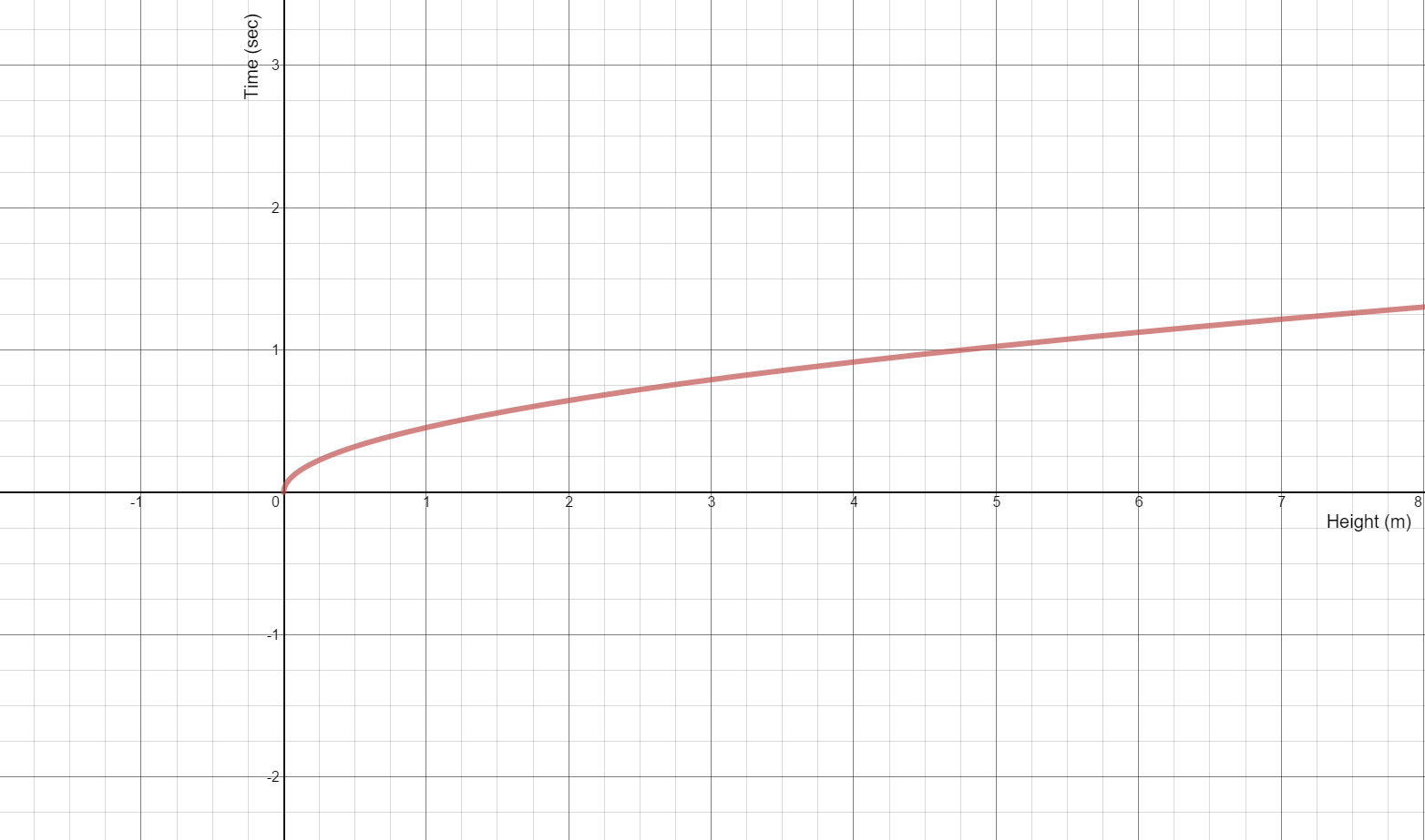
Now, given a measured time, , all one needs to do is draw a horizontal line on this plot at that value of time, find the intersection point with the curve shown, and read off the value of , the predicted depth of the well. It’s  worth a conversation as to whether or not the term is important here or when it may be important. It’s also worth taking time exploring how an error in the measurement of translates into an error in the prediction of . The sensitivity to such error that one sees in this problem is a typical feature of inverse problems.

If you do decide to introduce your students to the notion of inverse problems, it is worth spending at least a few minutes sharing with them the many areas of application where such problems arise. I’d suggest focusing on medical imaging as this is likely familiar territory in some sense, but unfamiliar territory in the sense of them understanding that most of modern medical imaging rests on building mathematical models and solving inverse problems.

I’ll leave you with one last inverse problem that is readily understood, but challenging to investigate. Imagine I tell you that I have a container of some sort but that I’m going to keep that container hidden in a box and not let you see it directly. However, what I will do is pour any volume of water you’d like into the container and tell you the height to which the water fills this hidden container for that volume. I’ll do this as many times as you’d like and give you as much data of this form as you want. The question is then this – can you tell me the shape of my container? Suppose I told you the container had rotational symmetry. Would that help?

I hope that this small taste of inverse problems has inspired you to consider this very important class of problems as you work to build mathematical modeling into your classroom practice. As always, we’d love to hear about your successes and challenges with this or other mathematical modeling investigations.

John

In a previous post we introduced the idea of a “toy model” in the context of investigating pollution in the Great Lakes. Today, I want to talk more about this idea of a “toy model,” explore a simple toy model that you can introduce in your classroom, and point you toward one resource that’s full of such ideas for students at the middle and high school level.

When a modeler approaches a problem in the real-world, they generally encounter something that is complicated, messy, and hard to get a handle on. It’s not clear what’s important and what’s not. It’s not clear what’s hidden underneath what can be observed and it’s often not clear where to even begin trying to understand what they’re seeing. There are many different approaches that modelers use when they find themselves at this point with a new problem. They may recall an analogous situation that seems similar enough to this new situation and use that observation as a starting point, trying to understand what’s different between what they see and what’s familiar. They may start with data and try and see what trends they notice or what patterns they can see from studying the data. Or, they might employ the mathematician’s strategy of what to do when faced with a problem where you don’t even know where to start – replace it with a simpler problem that you can solve but that is close enough to your original problem that you think you might learn something about solving the tough problem. When modelers use this strategy, they often say what they are doing is “considering a toy model” or “playing with a toy model.”

This strategy often leads to incredibly rich mathematics and insight into the real world problem. While you may still be many steps away from fully understanding the real world system, you’ve often found that path where at the very least you can start your journey. One beautiful example of this is what’s know as the Renyi Parking Problem. The Hungarian mathematician Alfred Renyi first posed this problem as a toy model of the more complicated problem of random packing. Random packing situations arise in many areas of scientific and industrial interest. When scientists investigate how molecules bind to the surface of some object, it’s really a random packing problem. When you ask the question “How many jellybeans are in this jar?” you are really asking a random packing question. The basic idea is simple – if you randomly place objects in some confined region of space, how much of that space will you fill up? What happens if those objects can push other objects that are already there around? What happens if sometimes an object leaves that space? You can imagine that the problem in any particular application can quickly seem complicated and overwhelming.

Renyi posed a simple to understand, but mathematically rich, toy model of random packing. He imagined a long street of some length, say L, where cars of unit length were allowed to park. He then asked “what happens if the cars park randomly in any unit interval that’s not already occupied along this street?” So, there’s no parking spaces, and the drivers are discourteous and don’t try and park close to other cars. The story of the investigation of this problem and open questions that still remain about it is quite interesting. But, here what we want to observe is what Renyi did. He didn’t take any particular real-world problem and make assumptions and abstractions and try and get to a problem he could mathematize. Rather, he simply posed a problem that he could easily mathematize, but had the “flavor” of the phenomena he as trying to understand. That’s the essence of constructing a toy model and part of the art of mathematical modeling. Often the modeler has to be able to “see through” all of the real-world complications to some underlying “toy” system that can be grasped, mathematized, and understood.

The book Adventures in Modeling by Colella, Klopfer, and Resnick is chock-full of examples of toy models that can readily be investigated in the classroom. The book focuses on exploring complex, dynamic systems and hand-in-hand introduces the reader to using StarLogo as a simple simulation tool. StarLogo is one of those programming environments that was specifically designed to be easy for students to learn and to serve as an entry point into computer programming. But, even if you ignore the StarLogo part of the book, the problems and the toy models introduced are alone worth the price.

One activity that they explore is called “Foraging Frenzy” and it’s a nice one for exploring mathematical modeling, toy models, and connecting your math classroom to biology and ecology. The underlying ecology problem is a central one to the field. How do you predict what an animal will do when foraging for food? You can imagine how complicated such a situation can get in context! Suppose we’re talking about field mice. How far will they roam? How will they decide? What happens if there are predators in the environment? How does their behavior depend on the season? Thought about in context, the problem is certainly one of those that can feel overwhelming. I’d even argue that it is one of those problems that if given directly to a group of students might very well end up with students saying “You can’t possibly predict what an animal will do when foraging for food!” So, what we often end up doing as teachers is just telling our students what happens and removing the whole exploration part from these complex problems. This is where I believe toy models can be very useful in the classroom.

What Colella et. al. do is to introduce a toy “foraging model” that does feel tractable and does feel like one where students can start seriously exploring and thinking about how to model. They say this – buy a big bag of dried kidney beans, get three stopwatches and a piece of paper. Now, assign two students to be “food givers” and give them each half of the beans and a stopwatch. Have them sit close to one another and secretly tell each of them the rate at which they are to give out their beans. For example, tell one student to give out a bean every five seconds and the other every fifteen seconds. Now, tell the rest of your students that their job is to get as many beans as they can, but they have to follow a few rules. They have to stand in line in front of one of the “food givers” and take a bean when it is given to them. They are allowed to switch lines at any time, but always must move to the back of the other line. After they get a bean they also must move to the back of one of the lines. Now, let them go! In the meantime, you’re using your stopwatch to gather data. Note the number people in each line at regular time intervals, say every 30 seconds. Let the whole process run for 5 minutes and then share what you’ve recorded with the class.

What you have presented students with is a really simple, accessible “toy model” of foraging behavior. It’s one for which you have data, is one that’s more manageable in scope, but also captures the essential features of the real-world ecological problem. Now, it’s time to discuss and think about modeling. If your students behave like many animals in the natural world, what you’ll see is that the length of lines becomes proportional to those rates of distribution that you set at the beginning. That’s something that’s called “Ideal Free Distribution” theory and is the basis for making those predictions about what a foraging animal will actually do.

I encourage you to make use of toy models liberally in your classroom as you introduce the notion of mathematical modeling. Let us know if you try this one out or come up with other neat “toy models.” We’d love to hear from you.

John

In his wonderful book, How Not to be Wrong: The Power of Mathematical Thinking, Jordan Ellenberg uses an excerpt from Mark Twain’s Life on the Mississippi to make an important point about fitting linear models to data. While Ellenberg’s book covers topics that extend well beyond mathematical modeling into areas one would commonly label as “quantitative reasoning,” he captures a heck of a lot about how modelers think and how a mathematical modeler approaches the world. Today, I want to borrow Ellenberg’s Mark Twain tale and discuss the importance of two words that appear in the CCSSM, namely, descriptive and analytic.

Let’s start with the excerpt from Twain’s Life of the Mississippi:

The Mississippi between Cairo and New Orleans was twelve hundred and fifteen miles long one hundred and seventy-six years ago. It was eleven hundred and eighty after the cut-off of 1722. It was one thousand and forty after the American Bend cut-off. It has lost sixty-seven miles since. Consequently its length is only nine hundred and seventy-three miles at present. . . . In the space of one hundred and seventy-six years the Lower Mississippi has shortened itself two hundred and forty-two miles. This is an average of a trifle over one mile and a third per year. Therefore, any calm person, who is not blind or idiotic, can see that in the Old Oolitic Silurian Period, just a million years ago next November, the Lower Mississippi River was upward of one million three hundred thousand miles long, and stuck out over the Gulf of Mexico like a fishing-rod. And by the same token any person can see that seven hundred and forty-two years from now the Lower Mississippi will be only a mile and three-quarters long, and Cairo and New Orleans will have joined their streets together, and be plodding comfortably along under a single mayor and a mutual board of aldermen. There is something fascinating about science. One gets such wholesale returns of conjecture out of such a trifling investment of fact.

Now, Mark Twain was a funny guy and, of course, this was intended to be a humorous passage. But, it also well-illustrates the dangers of “modeling without thinking” and that’s what I’d like to caution against here. What Mark Twain was implicitly engaging in was the practice of what the CCSSM calls descriptive modeling. And, that’s a useful and important practice, done right. But, it has its limitations and it is precisely these limitations that drive the need for what the CCSSM calls analytic modeling.

Let’s first make sure we understand Mark Twain’s analysis.  How might we approach this “Mississippi shrinking” problem from a purely descriptive point of view? Well, from the excerpt above and from doing a little digging as to when the American Bend cut-off occurred, we have four data points:

Year         Length (miles)
1716        1215
1722        1180
1858        1040
1883          973

It’s a simple matter to plot these data points and fit a line to our data:

If you click on the plot and examine it closely, you’ll see that we have an R-squared value of 0.9747! Well, that’s fantastic, it means more than 97% of the variance in our data is explained by our line! So, we have a mathematical model that tells us how the Mississippi is shrinking with time and we can now make predictions, right? Well, that’s really Mark Twain’s point. We can’t. In Life on the Mississippi, Twain extracted the slope of our line and found that according to our model, the Mississippi is losing about a mile and a third of length each year. In some sense, that’s right of course. But, in a more important sense, it is horribly wrong. The sense in which that’s wrong, is the sense in which descriptive mathematical modeling is limited, and is a tool that we have to wield very carefully. It’s also why, as mathematical modelers, we’re driven to seek the deeper sort of understanding that comes from analytic modeling.

The CCSSM has this to say about descriptive modeling:

In descriptive modeling, a model simply describes the phenomena or summarizes them in a compact form. Graphs of observations are a familiar descriptive model—for example, graphs of global temperature and atmospheric CO2 over time.

That’s a pretty good description of what Twain did in his passage. What’s important to note about descriptive modeling is that it is always an extra step removed from the real-world phenomena we are trying to understand. When we do descriptive modeling, what we’re actually doing is giving some shape to a data set. We’re describing that data, saying “this data looks like this function.” Yes, we make “looks like” very precise by doing what we call “regression,” but underneath, it’s still “this data looks like this function.” And, unless the underlying phenomena continues to behave exactly as it did when it provided our data set, our description won’t be useful for making predictions. That’s where we have to very carefully think things through. Do we have any reason to believe that the trend we see will continue? If so, how far? These are always questions we should be asking whenever we do descriptive modeling.

The CCSSM also talks about analytic modeling:

Analytic modeling seeks to explain data on the basis of deeper theoretical ideas, albeit with parameters that are empirically based; for example, exponential growth of bacterial colonies (until cut-off mechanisms such as pollution or starvation intervene) follows from a constant reproduction rate.

Teaching students to understand the difference between descriptive and analytic approaches is a crucial part of teaching the art of mathematical modeling. Descriptive modeling has its time and place and in many situations its the best we can do. But, I’d argue that we should always be pushing our students deeper, pushing them to question descriptive models carefully, and pushing them to really try and understand the world by developing their skills as analytic modelers.

John

Q: How did the chicken cross the road?

A: One step at a time. 

In various Twitter conversations with @Foizym, @ddmeyer, @MathMinds,  @gfletch, and @Simon_Gregg, the question of what mathematical modeling could or should look like at the elementary level has been a recurring theme. I want to explore this question a little bit in this post and offer a few ideas that may be helpful for those trying to incorporate mathematical modeling into their elementary math classrooms.

A good deal of the angst around teaching mathematical modeling at the elementary level seems to revolve around what it is that students already know. That is, they have a limited mathematical toolbox to draw from and a limited extra-mathematical toolbox to draw from. Put simply, there’s a lot they don’t yet know. And, I can’t argue with this as being a serious challenge. If the mathematics taught in K-8 was adequate for dealing with all the myriad problems that mathematical modelers attack, well, then we would never have needed to invent calculus, or differential equations, or algebraic topology, or… you get the idea.

And, it simply is true that the extent of the tools in your toolbox limits what projects you can successfully tackle. If all I have is a hammer and saw, it’s pretty hard to build a cathedral. If I really want to build a cathedral, I’ll probably spend a good deal of time using my hammer and saw to build other tools and then use those to build still other tools, and then get around to building a cathedral. The obvious analogy is that if I want to do mathematical modeling of fluid dynamics, and all I have is algebra, I would probably need to spend some time building calculus before I’d be able to get very far.

But, this, of course, is deeply unsatisfying. It almost kicks us back to the horrible answer to a students’ question of “what is this good for?” of “wait, you’ll see in a few years.” So, if we reject that answer, and yet realize that students at the elementary level do have a limited toolbox, what do we do? I’d like to offer two answers.

The first of these is that we can assiduously look for those problems that can be tackled with a limited toolbox. This is hard! Once you own a table saw, you’re not so likely to whip out your handsaw any more, so when we survey the scientific literature, we’re not so likely to find many problems that rely only on elementary mathematics. That doesn’t mean that they don’t exist nor that the problems we do find couldn’t also be attacked by elementary means, just that what we’re seeking won’t be sitting right on the surface for us to discover. It means that someone seeking to find good problems for elementary students will themselves have to be a pretty darn good modeler. They’ll have to not only be able to digest the modeling literature that uses advanced mathematics, but also be able to see how such problems could be attacked more simply, or how parts of those problems could be attacked using elementary math. That’s a tall order but I think this is a potentially useful approach. That is, I’m arguing that rather than try and construct elementary mathematical modeling projects from scratch, lets have elementary experts sit down with modelers, plow through some hard problems, and see what comes out the other side. Could such a team identify the accessible projects? I don’t know, but I think it is worth a try. I offer our previous discussion of “fairy circles,” albeit aimed at high school, as an example of what I mean here.

So, what’s the second answer? I’d argue that another approach we could take is to think really hard about why tools like calculus were developed in the first place. I’d argue that while much of the mathematical machinery used day-to-day by mathematical modelers is inaccessible to young students, a lot of the ideas behind that machinery are actually very accessible. The simplest and perhaps broadest example that occurs to me is the notion of iteration. Much of what we do in science and much of what we do as modelers is to build on a very simple idea that I’ll state like this – right now, the world looks exactly like it did a little bit ago, but with some tiny changes. That is, calculus, differential equations, and a whole bunch of the mathematical machinery that modelers rely on was built to be able to model change. And, the idea that is repeatedly used is the one we just stated, things change in small steps.

So, if I want to know how the chicken crossed the road, the useful answer is “one step at a time.” I then build up my understanding of “chicken crossing” from a chicken repeatedly executing single steps. If I do this over and over, I get my chicken where he wants to be. To see how we might follow this line of thinking to get from a “standard” calculus-based modeling topic down to the elementary level, let’s look at a simple, canonical mathematical model that you’ll see in any modeling textbook – population growth.

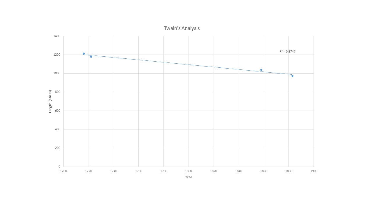
Typically, in studying population growth (or how the amount of any “stuff” increases or decreases with time), you’ll first examine linear growth. If is the amount of stuff at time , you’d write:

So, what are we really saying? Well, we’re saying that the rate of change of is a constant. We can view that differently if we approximate our derivative by it’s difference quotient:

Or, rearranging:

Now, what does this really say? Well, it says the amount of stuff we’ll have in the future, , is equal to the amount of stuff we have now, , plus a tiny change, . That is, in a little bit, the world looks just like it does now, with a tiny change. We do this repeatedly, and we get a picture of how our system changes according to the underlying process of changing by constant small steps.

Well, that’s not really very hard to grasp at all! So, imagine we introduced this idea to young students. Imagine we showed them a simple table of data that gave the population of something for different times. Maybe it looks like this:

Time    Population
0                 1
1                 2
2                 3

and so on… Often, we’ll give data like this and ask students to predict what comes next or to discover the pattern. Now, what we’re doing is asking them to guess at the underlying process leading to the data they see. If a student’s answer (model) looks like “the amount of stuff we have later is equal to the amount of stuff we have now plus a little bit,” that seems to me like a pretty powerful realization.

You can imagine then presenting students with different systems that change with time in different ways and have them engage in the modeling exercise of trying to understanding the key underlying process. Their model might be as simple as a written statement, but one they can test by doing repeated addition, subtraction, multiplication, and division. Heck, they might even start to wonder if their is a more convenient or powerful way to do this stuff…

I guess at the end of the day what we’re arguing is once again that mathematics is the science of pattern and mathematical modeling is about applying that science to patterns that occur in the real world. If we keep this in mind, and look for those patterns in the real world whose origin or dynamics can be explained by some iterative process that at its heart consists of addition, subtraction, multiplication, and division, we might indeed be able to engage students at all levels in genuine, interesting, engaging mathematical modeling investigations.

John

Last time, we introduced the fairy circles of Namibia and talked about the idea of self-organization as a possible explanation. In case you’ve forgotten, these are bare patches in the desert, roughly circular, roughly the same size, that form over a huge swath of land. They look like:

Fairy circles

We talked about recent attempts to explain these circles using a mathematical modeling approach and noting that current models are well, complicated mathematically. We ended with the claim that yet, this might just be a good modeling investigation for the high school classroom.

So, today, I want to follow that thread and think about how your students might get a handle on this problem and what type of investigation they might be able to carry out. Here, I’m going to argue that this is a problem where a fairly simple model can be proposed, but that what’s essential to making it accessible is having students carry out the “analysis” of the model via simulation.

Let’s think about the fairy circles again for a moment. If you read the Ecography paper we mentioned last time or even if you just read the summary in Science News, you quickly get a sense that the main proposed driver of the growth of fairy circles is competition between plants for the scarce resource of water. There’s more to it than this, but as a modeler, it’s worth ignoring all the complications and just thinking through this simple bit a little more. Remember, when we’re doing mathematical modeling, part of our job is to do what we’re doing here – make a guess about what we think is driving what we see, and then build a model around the guess. If our model reproduces what we see based on this driver, we have a little more evidence that our guess is the correct one. If not, we iterate!

So, suppose we have a whole bunch of randomly dispersed plants in some region. Perhaps the situation looks something like this:

To create this picture, I choose 3010 points at random in a restricted subset of the plane. I then plotted small dots at 3000 of these points. At the other 10 points, I plotted larger, red dots. What I’m imagining here is that we have a bunch of randomly dispersed plants and that most of these are “small” plants, i.e. the 3000 dots. The other 10 plants are “large” plants. They are going to be a bit special.

Now, what I imagine next is that as time evolves, each small plant has some probability of dying. Nothing special at all so far! We have a bunch of plants and over time, they can die. Here’s where we are going to introduce this idea of competition. Suppose the probability of a small plant dying is inversely proportional to how far it is from the nearest big plant. So, we’re saying that if I’m close to a big plant, it’s going to suck up all the water and I’m more likely to die. Well, if then let time proceed in discrete steps, at each time step rolled a die to see whether or not each plant in our picture lives, and removed the dead ones from our picture, we could then see whether or not a pattern of bare spots evolves in our system. Designing a simulation to do this would be a test of our model and a test of our hypothesis that it’s this form of competition creating fairy circles.

Note that we’re not using very sophisticated mathematics at all right now. Let’s be really explicit about what our model looks like. Here it is:

(1) We assume that there are two types of plants in our system, “big” and “little.”

(2) We assume our plants are randomly distributed in some fixed region.

(3) We assume time can be modeled as proceeding in discrete steps.

(4) With each small plant, we associate a probability of dying that is inversely proportional to its distance from the nearest big plant.

(5) We let time proceed in our system, rolling a theoretical die to determine whether or not each small plant dies during that time step, and remove it from the picture if it does.

(6) After awhile, we look at our picture and see if any patterns emerge.

Now, in a second I’ll show you what doing this looks like and talk a bit more about the simulation. But, first, let me note that you can explore this idea of pattern formation in  a really simple way in your classroom. Imagine literally doing this with your students. Literally. That is, suppose you identified the student in the middle of your classroom as the “big” plant. Then, assign students probabilities that depend on how close they sit to this “big” plant student. Now, generate random numbers, and have those students who “die” get up and walk to the back of the room. If you do this for a few iterations, what does the space defined by the empty seats look like?

Well, when you do this with the 3010 plants in the above picture, after a few iterations, you see the following:

Huh. We have bare patches, roughly circular, that kind of look like fairy circles! So, how we solved the mystery? Well, no. Note that there is a really important difference between our fairy circles and the ones we see in nature. Our circles all have a live plant smack dab in the middle of them! We’ve really shown how fairy donuts might form, rather than fairy circles. Well, this is quite interesting and begins to suggest to us that the competition driving the formation of fairy circles might be a little more complicated or subtle than we first supposed. At the same time, it nicely highlights why mathematical modeling is an iterative process. We started with an observation, made a guess about what drove what we saw, built a model around that guess, analyzed the model through simulation, and then compared the results of our analysis with our original observation. The difference between what our analysis led to and what we originally observed now forces us to modify our guess, improve our model, and… around we go again.

While I don’t know that your students will be able to totally solve the fairy circle mystery, I can easily imagine that they can carry out an investigation like this one. Going around the modeling cycle together a few times in an investigation like this one, seems quite worthwhile. You may not get to the “end” or completely solve the mystery, but I hope that will serve as a reminder that all science is provisional, that these investigations build over time, that we learn a bit at each step, and that a lot of the real fun comes in the investigation rather than the solution.

So, to carry out this type of investigation, it’s obviously important that students have the ability to sketch out and quickly use a simulation tool. As I’ve mentioned before, there are many free options that lets students do this. For this particular one, I used one of my favorites, an open-source, easy to use, but powerful language called Processing. I’ll paste my Processing code below in case you want to give it a try. As always, let me know if you want to talk fairy circles some more. We’re always happy to help and talk more about modeling.

John

Processing Code – Uses Processing 3

//Sketch to simulate proposed mechanism for Fairy Circles
//John A. Pelesko, 8/24/2015

void setup()
{
//Create the space we will work in.
size(500,500);
background(255);
//Create a 2-dimensional array for our “big” plants
int colBig=2;
int rowBig=10;
int[][] BigPlants = new int[colBig][rowBig];
for(int i=0; i<colBig; i++)
{
for(int j=0; j<rowBig; j++)
{
float r = random(500);
int s = int(r);
BigPlants[i][j]=s;
}
}

//Now display Big Plants as large ellipses
for(int j=0; j<rowBig; j++)
{
fill(250,5,21);
ellipse(BigPlants[0][j], BigPlants[1][j], 15, 15);
}

//Create a 2-dimensional array for our “little” plants
int colSmall=3;
int rowSmall=3000;
int[][] SmallPlants = new int[colSmall][rowSmall];
for(int j=0; j<rowSmall; j++)
{
float r1 = random(500);
float r2 = random(500);
int s1 = int(r1);
int s2 = int(r2);
SmallPlants[0][j]=s1;
SmallPlants[1][j]=s2;
SmallPlants[2][j]=1;
}

//Now display Small plants as small ellipses
for(int j=0; j<rowSmall; j++)
{
fill(15,15,15);
ellipse(SmallPlants[0][j], SmallPlants[1][j], 5, 5);
}

//Save a picture of where we start
save(“startingconfig.jpg”);

//For our small plants we have included a third column of data
//The 3rd column will be the state variable with 0=dead, 1=alive

//Setup an array to hold distances that we compute and probabilities
//To compute the values for the probabilities, we want to find the distance between a given small plant and each large plant
//Then, we take the smallest distance and set the probability of death as exp(-a*distance)
//The parameter a is an adjustable competition factor
float[] distarray = new float[rowBig];
float[] probarray = new float[rowSmall];

//Now, loop through each row of the array of small plants, for each row, compute distance to each big plant and store
for(int j=0; j<rowSmall; j++)
{
for(int i=0; i<rowBig; i++)
{
float xdif = sq((SmallPlants[0][j]-BigPlants[0][i]));
float ydif = sq((SmallPlants[1][j]-BigPlants[1][i]));
distarray[i] = sqrt(xdif+ydif);
}

//Find shortest distance in distarray
float s = min(distarray);
//Set probability for jth small plant
float prob = exp(-0.01*s);
probarray[j] = prob;
}

//Now, evolve the system
int timesteps = 3;
for(int i=0; i<timesteps; i++)
{
for(int j=0; j<rowSmall; j++)
{
float r1 = random(1);
if(r1<probarray[j])
{
SmallPlants[2][j]=0;
}
}
}

//Finally, display evolved system, only showing live plants
background(255);
for(int j=0; j<rowBig; j++)
{
fill(250,5,21);
ellipse(BigPlants[0][j], BigPlants[1][j], 15, 15);
}

for(int j=0; j<rowSmall; j++)
{
if(SmallPlants[2][j]==1)
{
fill(15,15,15);
ellipse(SmallPlants[0][j], SmallPlants[1][j], 5, 5);
}
}

//Save a picture of where we end
save(“endingconfig.jpg”);

}

Mathematics is the science of pattern and when we are doing mathematical modeling, we’re extending or tying the investigation of pattern explicitly to patterns in the real world. These might not be clear, simple, spatial patterns like those that usually occur to us when we hear the word “pattern.” They might be patterns in time, or patterns in some observed data set. But, sometimes, like in the case of the so-called “Fairy circles of Namibia,” they just might be clear, simple to observe, spatial patterns in nature.

Recently, these fairy circles were back in the news due to an article about their origin that appeared in Ecography. Science News published a short piece on fairy circles, covering a bit of the history of the search for an explanation, and an update on recent thinking. Their article, titled “What fairy circles can teach us about science,” got me to wondering what fairy circles might teach us about mathematical modeling.

So, today, I’d like to explore fairy circles, how we might approach this phenomena as a mathematical modeler, and hopefully demonstrate how a question still open to modern science can be accessible to investigation in the high school math classroom. I want to do this in some detail, so, fair warning, this will be a multi-post sort of investigation.

Let’s start by just looking at fairy circles. Following is a picture of the phenomena from an article by CNN addressing the topic. You can find plenty of such pictures with a simple Google of “fairy circle Namibia.”

Fairy circles

I think the picture makes the basic phenomena quite clear. You’re looking at a section of desert, where the green is plant life, and the open circles are simply bare spots, devoid of plants. These circles dot the landscape of a 2000 km long strip of desert, each circle somewhere between 5 m and 10 m in diameter, and the circles grow, shrink, disappear, and reappear in time. The question of course is – why the heck are there bare circles?

They get their name of “fairy circles” from the explanation that they are created by gods, spirits, or fairies. The image of thousands of fairies deciding to take a break, landing in the desert, and creating a nice little circular clearing for themselves is an appealing one. Over time however, various alternative theories have been proposed. These include toxic soil, termites, and radioactivity. They also include the idea that these patches are the result of self-organization, and that they occur naturally as the result of competition for scarce water resources between plants in the desert. This is the hypothesis that I’d like to investigate here.

The idea of self-organized pattern formation is generally attributed to Alan Turing. Yes, the same guy that cracked the Enigma machine, invented the computer, and who was so ably portrayed by Benedict Cumberbatch in The Imitation Game.  (If you haven’t seen it, great movie!) Among other things, Turing was interested in patterns that occurred in living systems. That is, things like the stripes on a zebra or the spots on leopard. In a paper called “The Chemical Basis of Morphogenesis,” he showed how the processes of chemical reaction and diffusion could combine, under the right circumstances, to create sharp spatial patterning. This early paper triggered years of investigations by scientists into pattern formation based on this mechanism and related mechanisms. The mathematician Jim Murray captured a huge amount of this work in his excellent book “Mathematical Biology.” Now, the first point I want to make is that Turing’s investigation, and most of the subsequent investigations into pattern formation have been carried out via mathematical modeling. This area of pattern formation in living systems, given that mathematics is the science of pattern, has been an incredibly ripe and fruitful area for the mathematical modeler.

So, back to Namibia. When a mathematical modeler sees a spatial pattern, like fairy circles, they think “self-organization.” Now, what does that mean? Well, in general, that means they are inclined to look for some underlying physical mechanism, usually some form of competition between effects or between things, and then to see if this mechanism can indeed drive the system toward forming a pattern spontaneously. From the work of Turing and all those who followed him, they know that this isn’t unlikely. In fact, they know that lots of spatial patterns in nature, from the stripes on a zebra to the patterns created by the growth of bacteria in a Petri dish can be understood in this way. So, seeing fairy circles and hearing the hypothesis of self-organization as an explanation is a perfectly reasonable thing for the modeler. Their job is to then see if they can test this hypothesis by mathematizing the proposed underlying physical mechanism, and then analyzing the mathematical model to determine if there are conditions under which spatial patterns will indeed form. In this way, they are testing the hypothesis that the proposed physical mechanism can lead to the patterns observed. If their model can be shown to not lead to pattern formation, then they’ve ruled out the proposed mechanism as the sole cause of the patterns. If it can be shown to lead to pattern formation, then the mathematical conditions under which this happens can be checked against the real world, either strengthening the case for the proposed mechanism or suggesting refinements to the model.

This is the approach taken by Getzin et. al. in the Ecography paper mentioned above. They’ve built a mathematical model that “supports the hypothesis that fairy circles are self-organized vegetation patterns that emerge from positive biomass-water feedbacks involving water transport by extended root systems and soil-water diffusion.” Okay, that’s a mouthful, and their mathematical model is pretty darn sophisticated. It’s a system of non-linear partial integro-differential equations for… well, it’s complicated. So, why would I claim this is a problem appropriate for the high school classroom?

Ah! That’s a pretty good cliff-hanger, so let’s break here for today and pick up next time with this question. In the meantime, perhaps you might think about how your students might think about this problem. That is, suppose you told them about fairy circles and that competition between plants was a proposed mechanism behind the patterns. How might they investigate this through mathematical modeling? How might you? Till next time…

John

Back in “Curiosity, golf math, and another tool for your classroom,” we explored the high-speed video capabilities of the iPhone 6 and talked about how we might use this tool to develop interesting mathematical modeling problems. High speed photography, like that of the iPhone, lets us “see fast.” That is, we can use that tool to see things that happen more quickly than we can ordinarily perceive.

Well, the iPhone (and iPad, and iPod touch) lets us go in the other direction as well. We can take advantage of the time-lapse photography mode and see slow. That is, we can capture things that happen so slowly that the change is not within our typical perception of events.

One of my favorite summertime “seeing slow” things to do is to get up early and watch the sunrise over the ocean. This year, I was fortunate to have a chance to spend a few days in Cape May, NJ, with beautiful weather, and plenty of opportunities to watch the sunrise. I decided to take this opportunity to explore the time-lapse capabilities of the iPhone and to think a bit about how we might use time-lapse video to create mathematical modeling opportunities in the classroom. Here’s one video I took that spans about 30 minutes of real-time and 27 seconds of “time-lapse” time:

In time-lapse mode, the iPhone dynamically chooses the frames per second captured for a time-lapse video, with the frame rate dependent on the total length of the video. For a video that is between 20 and 40 minutes long, like this one, it takes one frame per two seconds and then speeds up the playback time to 60 times normal speed. If the normal playback speed in 30 frames per second, it is now playing the equivalent of 1800 frames per second, so we see 60 seconds of real time for every one second of video. That’s what you are watching in this video.

Now, watching the sun rise like this got me to wondering – how many students have actually seen the sun rise? How many have thought about how “brightness” changes as we go from dark to light? If I asked my students to plot “brightness” versus time as we transitioned from before sunrise to after, what would their plots look like? If you get a chance to ask your students this question, please share their thinking!

In the meantime, let’s see what we can actually learn about how brightness changes using our time-lapse video of a real sunrise. Along the way, we’ll learn a little bit about image processing, and pick up a few more tools for you and your students to use during your investigations.

We’ve already seen how easy it is to collect data using an iPhone or similar device in the form of video. The problem is that video isn’t the most convenient format to use when what we want is numerical data. It is generally much easier to extract numerical data from a still photo. So, the first thing we need to do is extract individual frames from our video. Fortunately, this is pretty easy and you can do the job with a free piece of software called VLC Media Player. It’s ad free, easy to use, and available for just about any operating system you choose. You can easily find instructions as to how to do the frame extraction from video, so I’ll let you read about that elsewhere. This web page is a good start.

The more interesting question is what to do with the still photographs once you have them. This is where we need to do a little image processing and to do that it’s helpful if we know how to do a little coding. In fact, knowing how to do a little coding is pretty much an essential skill for the mathematical modeler. At the very least, being able to do a little coding vastly extends the range of what you can do with your mathematical models and for models that are mathematically complex, being able to code and obtain a numerical solution to your problem is often the only path forward. So, I’d advocate having your students learn to tap into the power of computing every chance you get! There are an incredible number of programming languages available now, many designed for the first time coder and for very young students, so this isn’t nearly as challenging as it was even twenty years ago. I’d urge you to spend a little time playing with languages like Scratch and the one we’ll use today, Processing.

Here, I’m going to advocate using Processing because it is open-source (free!), easy to learn, and powerful enough for just about anything you might want to do. It’s also the platform for the language used by the Arduino, so learning Processing also gives you access to playing with microcontrollers and extends your range in that dimension as well.

Now, to do our image processing, all we need to do is load individual images using a simple Processing sketch and then use the built-in function “brightness” to read off the brightness of selected pixels in our image. I selected 7 frames from the video above, evenly spaced in time, selected 5 pixels in each frame, and determined an average brightness for the image by averaging the brightness of each of those 5 pixels. That is, I did this quick and dirty. If you do this with your students, this is a good point to have a conversation about which pixels to select, how to select them, how many to select, and so on. But, for our purposes here today, this let me quickly make a plot of how the brightness of the beach during our sunrise changed with time. Here’s what my plot looks like:

Note that the frames I selected, again evenly spaced in time, span the entire period from “dark” to “light” in the video above. Now also note, we’ve taken the video and our qualitative view of “things getting brighter” and extracted quantitative information that we can start thinking about and playing with.

As soon as we see this plot, we start to wonder – Why does it have this shape? Boom! There’s a modeling problem. We’ve taken an observation about a pattern (it gets brighter outside as the sun rises), and turned it into something quantitative that we can now try and explain. We can ask plenty of related questions here. Can we explain this data based on what we know about how the Earth rotates? What would this data look like if we followed it for the whole day? Several days? A year? What would the data look like if the Earth were flat and the sun revolved around the Earth? What would this curve look like if we were in Alaska? Or, in Arizona?

If you wanted to move from the sort-of “hey I went on vacation and noticed this” kind of motivation for this investigation to something more practical, you don’t even have to work very hard. Understanding how brightness varies where you are is, of course, essential to understanding whether or not solar energy is a viable alternative energy source for you. Google has actually recently launched “Project Sunroof,” where they are developing a “solar recommendation calculator,” based in-part, on precisely this type of information. Having your students model how the brightness of the day changes can be both fun and eminently practical.

So, you have a few more potential tools for your classroom as you work to incorporate mathematical modeling into your teaching – time-lapse photography, image processing, simple coding and perhaps inspiration to build a modeling investigation around sunrises or solar energy. If you want to explore any of these in more detail, drop me a line. I’m happy to talk more or help in any way I can. In the meantime, I hope you enjoyed contemplating the sunrise in a new way.

John

The other day, the science news web site, sciencealert.com, posted one of the great “science rants” of all time. It occurred during an interview with the late Richard Feynman, when he was asked a seemingly innocuous question about magnets. It’s worth the 7 1/2 minutes of your life it takes to watch:

Notice that in this clip, Feynman is talking about why questions. As we’ve mentioned before, these are the types of questions that are of concern to the mathematical modeler. We create mathematical models to explain or predict phenomena in the natural world. That is, the mathematical modeler is a scientist asking “why?” and “how?”, but a scientist whose primary tools are those of mathematics.

Feynman’s rant provides a fascinating glimpse into the mind of one of histories greatest scientists and his focus on “why?” makes this a must-watch for the developing mathematical modeler. So, today, I’ll just leave you with some questions to reflect on after you’ve watched Feynman’s rant:

What is Feynman saying about the nature of assumptions? Where is he talking about implicit assumptions? Where do these arise in the modeling process?

What is Feynman trying to say about the nature of “why” questions asked by scientists? How does this relate to the types of answers that are acceptable for a particular “why” question?

Feynman makes some very careful points about the nature of explanation and “cheating” with an explanation. What is he trying to say? How does this relate to explanation through mathematical modeling?

I hope you enjoy this particular clip. We’re fortunate to live in an age where we have access to great minds like Feynman’s, even after they’ve left us. I encourage you to take advantage of that and perhaps spend some time following the YouTube thread through Feynman’s interviews and lectures.

– John

Last week, after the post about the “tipping buckets” problem, I heard from a really wonderful high school mathematics teacher who works here in Delaware. She had some really nice ideas about how to adapt and use this problem in a unit about linear and piecewise linear functions. This got me thinking…her approach to developing modeling activities was exactly the right way to do things. She was starting with the science, not the math.

Teachers working to implement mathematical modeling in their classrooms for the first time often, understandably, have the opposite instinct. That is, it is tempting to look at your syllabus or textbook topic by topic and think “How could I find a modeling problem that fits into this particular topic?” Teachers who push forward with that strategy often then find their problems feeling “forced” or contrived, and are disappointed when their students don’t end up excited by the activity. I’d argue that with this approach, that is, starting with the math and then finding the science, you’re more likely to end up with forced or contrived problems and to lose the whole sense of excitement and investigation that should accompany modeling activities.

Now, this is not to say that the strategy of “math first, then science” can’t work. In fact, I think it can work if you have a huge library of modeling problems in your head. Someone who has been engaged in mathematical modeling for a long time, can typically look at a topic and say “Oh, I know a neat problem that naturally leads to the study of…” But, for someone who is just starting out, and who doesn’t yet have this library, approaching things this way seems to, well, not work out very well.

So, instead, if you’re just starting out as a learner and teacher of mathematical modeling, I’d advocate you try the approach that our Delaware teacher took. Keep your eyes open, wade through STEM activities, see what your neighborhood science teacher is up to, visit science fairs and science museums, and approach what you see as a mathematical modeler. Would a mathematical model help me explain and understand what I’m observing? Would it help me predict what will happen next? As soon as the answer becomes “yes” to either or both of those questions, the mathematics will leap into your mind and you’ll know where in your curriculum an activity based on this idea would fit. And, it will fit naturally, the science will be genuine, and students will respond better to this authenticity.

Okay, these are all fine words, but I personally would be more convinced by an example. So, as I thought this notion of “start with the science, not with the math” through, I decided to try it out for myself, and see how well it worked. I started by Googling “STEM activities” and went from there. I quickly found myself at tryengineering.org, a really cool website that I highly recommend visiting. On their front page, you’ll find a link to 116 downloadable lessons plans in PDF format. You can search by age range and topic.

One of the first projects that caught my eye was “Water Rocket Launch,” a project that has teams of students learning about rocketry, engineering design, and building and launching their own water rockets. If you poke around on the web, you can find lots of sites with instruction and videos on water bottle rockets. They all basically look like and work like this one:

Now, going back to the activity at tryengineering.org, if you read through their lesson plan, you’ll see lots of engineering, lots of science, and even a little math thrown in when discussing Newton’s Laws. But, students are never asked or inspired to actually use math in any non-trivial way during this activity. Here’s where you come in! Why not do this activity in math class, or team up with your local science teacher and do it jointly, but carefully add in some mathematical modeling. The math you can incorporate ranges from simple applications problems like “How high did the rocket actually go?” where you can have students use a little trigonometry and one of these:

to challenging modeling problems like “How high could a water rocket possibly go?” Why not ask your students to predict how high their rocket will fly before they launch it? Why not make it a competition with prizes to the team with the highest flying rocket and to the team with the most accurate mathematical model predicting flight height? In doing any of this, not only are you bringing the use of mathematics into a cool STEM lesson plan, you’re bringing the lesson plan much closer to mirroring what STEM professionals actually do.

So, as you continue to work to incorporate the process of mathematical modeling into your classroom, keep the idea “start with the science, not the math” in mind. I think it’ll lead to less frustration and more success. Good luck!

– John