Last time, we introduced the fairy circles of Namibia and talked about the idea of self-organization as a possible explanation. In case you’ve forgotten, these are bare patches in the desert, roughly circular, roughly the same size, that form over a huge swath of land. They look like:
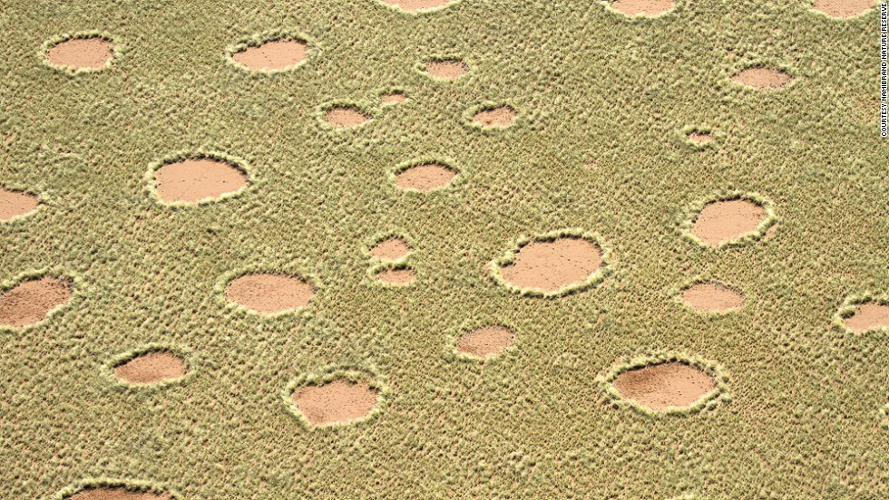
Fairy circles
We talked about recent attempts to explain these circles using a mathematical modeling approach and noting that current models are well, complicated mathematically. We ended with the claim that yet, this might just be a good modeling investigation for the high school classroom.
So, today, I want to follow that thread and think about how your students might get a handle on this problem and what type of investigation they might be able to carry out. Here, I’m going to argue that this is a problem where a fairly simple model can be proposed, but that what’s essential to making it accessible is having students carry out the “analysis” of the model via simulation.
Let’s think about the fairy circles again for a moment. If you read the Ecography paper we mentioned last time or even if you just read the summary in Science News, you quickly get a sense that the main proposed driver of the growth of fairy circles is competition between plants for the scarce resource of water. There’s more to it than this, but as a modeler, it’s worth ignoring all the complications and just thinking through this simple bit a little more. Remember, when we’re doing mathematical modeling, part of our job is to do what we’re doing here – make a guess about what we think is driving what we see, and then build a model around the guess. If our model reproduces what we see based on this driver, we have a little more evidence that our guess is the correct one. If not, we iterate!
So, suppose we have a whole bunch of randomly dispersed plants in some region. Perhaps the situation looks something like this:
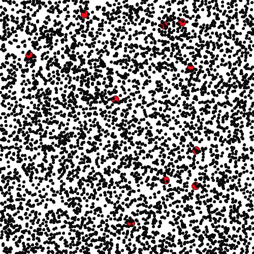
To create this picture, I choose 3010 points at random in a restricted subset of the plane. I then plotted small dots at 3000 of these points. At the other 10 points, I plotted larger, red dots. What I’m imagining here is that we have a bunch of randomly dispersed plants and that most of these are “small” plants, i.e. the 3000 dots. The other 10 plants are “large” plants. They are going to be a bit special.
Now, what I imagine next is that as time evolves, each small plant has some probability of dying. Nothing special at all so far! We have a bunch of plants and over time, they can die. Here’s where we are going to introduce this idea of competition. Suppose the probability of a small plant dying is inversely proportional to how far it is from the nearest big plant. So, we’re saying that if I’m close to a big plant, it’s going to suck up all the water and I’m more likely to die. Well, if then let time proceed in discrete steps, at each time step rolled a die to see whether or not each plant in our picture lives, and removed the dead ones from our picture, we could then see whether or not a pattern of bare spots evolves in our system. Designing a simulation to do this would be a test of our model and a test of our hypothesis that it’s this form of competition creating fairy circles.
Note that we’re not using very sophisticated mathematics at all right now. Let’s be really explicit about what our model looks like. Here it is:
(1) We assume that there are two types of plants in our system, “big” and “little.”
(2) We assume our plants are randomly distributed in some fixed region.
(3) We assume time can be modeled as proceeding in discrete steps.
(4) With each small plant, we associate a probability of dying that is inversely proportional to its distance from the nearest big plant.
(5) We let time proceed in our system, rolling a theoretical die to determine whether or not each small plant dies during that time step, and remove it from the picture if it does.
(6) After awhile, we look at our picture and see if any patterns emerge.
Now, in a second I’ll show you what doing this looks like and talk a bit more about the simulation. But, first, let me note that you can explore this idea of pattern formation in a really simple way in your classroom. Imagine literally doing this with your students. Literally. That is, suppose you identified the student in the middle of your classroom as the “big” plant. Then, assign students probabilities that depend on how close they sit to this “big” plant student. Now, generate random numbers, and have those students who “die” get up and walk to the back of the room. If you do this for a few iterations, what does the space defined by the empty seats look like?
Well, when you do this with the 3010 plants in the above picture, after a few iterations, you see the following:
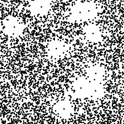
Huh. We have bare patches, roughly circular, that kind of look like fairy circles! So, how we solved the mystery? Well, no. Note that there is a really important difference between our fairy circles and the ones we see in nature. Our circles all have a live plant smack dab in the middle of them! We’ve really shown how fairy donuts might form, rather than fairy circles. Well, this is quite interesting and begins to suggest to us that the competition driving the formation of fairy circles might be a little more complicated or subtle than we first supposed. At the same time, it nicely highlights why mathematical modeling is an iterative process. We started with an observation, made a guess about what drove what we saw, built a model around that guess, analyzed the model through simulation, and then compared the results of our analysis with our original observation. The difference between what our analysis led to and what we originally observed now forces us to modify our guess, improve our model, and… around we go again.
While I don’t know that your students will be able to totally solve the fairy circle mystery, I can easily imagine that they can carry out an investigation like this one. Going around the modeling cycle together a few times in an investigation like this one, seems quite worthwhile. You may not get to the “end” or completely solve the mystery, but I hope that will serve as a reminder that all science is provisional, that these investigations build over time, that we learn a bit at each step, and that a lot of the real fun comes in the investigation rather than the solution.
So, to carry out this type of investigation, it’s obviously important that students have the ability to sketch out and quickly use a simulation tool. As I’ve mentioned before, there are many free options that lets students do this. For this particular one, I used one of my favorites, an open-source, easy to use, but powerful language called Processing. I’ll paste my Processing code below in case you want to give it a try. As always, let me know if you want to talk fairy circles some more. We’re always happy to help and talk more about modeling.
John
Processing Code – Uses Processing 3
//Sketch to simulate proposed mechanism for Fairy Circles
//John A. Pelesko, 8/24/2015
void setup()
{
//Create the space we will work in.
size(500,500);
background(255);
//Create a 2-dimensional array for our “big” plants
int colBig=2;
int rowBig=10;
int[][] BigPlants = new int[colBig][rowBig];
for(int i=0; i<colBig; i++)
{
for(int j=0; j<rowBig; j++)
{
float r = random(500);
int s = int(r);
BigPlants[i][j]=s;
}
}
//Now display Big Plants as large ellipses
for(int j=0; j<rowBig; j++)
{
fill(250,5,21);
ellipse(BigPlants[0][j], BigPlants[1][j], 15, 15);
}
//Create a 2-dimensional array for our “little” plants
int colSmall=3;
int rowSmall=3000;
int[][] SmallPlants = new int[colSmall][rowSmall];
for(int j=0; j<rowSmall; j++)
{
float r1 = random(500);
float r2 = random(500);
int s1 = int(r1);
int s2 = int(r2);
SmallPlants[0][j]=s1;
SmallPlants[1][j]=s2;
SmallPlants[2][j]=1;
}
//Now display Small plants as small ellipses
for(int j=0; j<rowSmall; j++)
{
fill(15,15,15);
ellipse(SmallPlants[0][j], SmallPlants[1][j], 5, 5);
}
//Save a picture of where we start
save(“startingconfig.jpg”);
//For our small plants we have included a third column of data
//The 3rd column will be the state variable with 0=dead, 1=alive
//Setup an array to hold distances that we compute and probabilities
//To compute the values for the probabilities, we want to find the distance between a given small plant and each large plant
//Then, we take the smallest distance and set the probability of death as exp(-a*distance)
//The parameter a is an adjustable competition factor
float[] distarray = new float[rowBig];
float[] probarray = new float[rowSmall];
//Now, loop through each row of the array of small plants, for each row, compute distance to each big plant and store
for(int j=0; j<rowSmall; j++)
{
for(int i=0; i<rowBig; i++)
{
float xdif = sq((SmallPlants[0][j]-BigPlants[0][i]));
float ydif = sq((SmallPlants[1][j]-BigPlants[1][i]));
distarray[i] = sqrt(xdif+ydif);
}
//Find shortest distance in distarray
float s = min(distarray);
//Set probability for jth small plant
float prob = exp(-0.01*s);
probarray[j] = prob;
}
//Now, evolve the system
int timesteps = 3;
for(int i=0; i<timesteps; i++)
{
for(int j=0; j<rowSmall; j++)
{
float r1 = random(1);
if(r1<probarray[j])
{
SmallPlants[2][j]=0;
}
}
}
//Finally, display evolved system, only showing live plants
background(255);
for(int j=0; j<rowBig; j++)
{
fill(250,5,21);
ellipse(BigPlants[0][j], BigPlants[1][j], 15, 15);
}
for(int j=0; j<rowSmall; j++)
{
if(SmallPlants[2][j]==1)
{
fill(15,15,15);
ellipse(SmallPlants[0][j], SmallPlants[1][j], 5, 5);
}
}
//Save a picture of where we end
save(“endingconfig.jpg”);
}
John – I wonder if you saw this wonderful post on unsolved mathematical problems, in which fairy circles are mentioned. https://liorpachter.wordpress.com/2015/09/20/unsolved-problems-with-the-common-core/
I had missed that one! Great post, thanks for sharing.
Hey very interesting blog!
Saved as a favorite, I really like your blog!